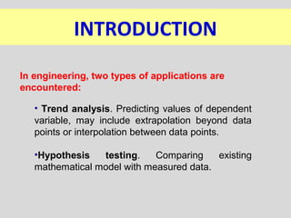
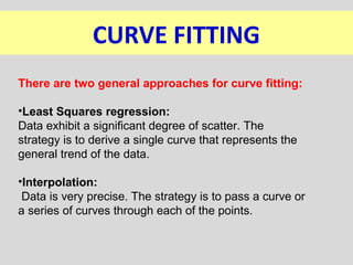
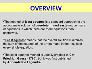
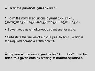
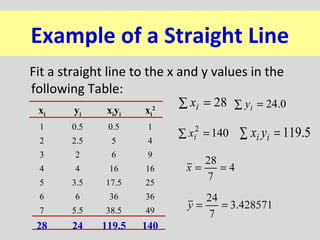
The document discusses the method of least squares for fitting curves to data points. It begins by introducing trend analysis and hypothesis testing as two applications of curve fitting. It then describes least squares regression and interpolation as two approaches for curve fitting. The main part of the document provides details on the least squares method, including forming normal equations from the data points, solving the normal equations to determine the coefficients of the curve, and examples of fitting straight lines and parabolas to data. It concludes by noting the key application of data fitting to minimize residuals and limitations when there is uncertainty in the independent variable.

1. METHOD OF LEAST
SQUARES
By: Varun Luthra
11CSU163

2. INTRODUCTION
In engineering, two types of applications are
encountered:
• Trend analysis. Predicting values of dependent
variable, may include extrapolation beyond data
points or interpolation between data points.
•Hypothesis testing. Comparing existing
mathematical model with measured data.

3. CURVE FITTING
There are two general approaches for curve fitting:
•Least Squares regression:
Data exhibit a significant degree of scatter. The
strategy is to derive a single curve that represents the
general trend of the data.
•Interpolation:
Data is very precise. The strategy is to pass a curve or
a series of curves through each of the points.

4. OVERVIEW
•The method of least squares is a standard approach to the
approximate solution of overdetermined systems, i.e., sets
of equations in which there are more equations than
unknowns.
•"Least squares" means that the overall solution minimizes
the sum of the squares of the errors made in the results of
every single equation.
•The least-squares method is usually credited to Carl
Friedrich Gauss (1795), but it was first published
by Adrien-Marie Legendre.

5. Scatter Diagram:
To find a relationship b/w the set of paired observations
x and y(say), we plot their corresponding values on the
graph , taking one of the variables along the x-axis and
other along the y-axis i.e. (X
1,y1),(x2,y2)…..,(xn,yn).
The resulting diagram showing a collection of dots is
called a scatter diagram. A smooth curve that
approximate the above set of points is known as the
approximate curve.

6. WORKING PROCEDURE
 To fit the straight line y=a+bx
 Substitute the observed set of n values in this equation.
 Form the normal equations for each constant i.e.
∑y=na+b∑x, ∑xy=a∑x+b∑x2
.
 Solve these normal equations as simultaneous equations of
a and b.
 Substitute the values of a and b in y=a+bx, which is the
required line of best fit.

7.  To fit the parabola: y=a+bx+cx2
:
 Form the normal equations ∑y=na+b∑x+c∑x2
,
∑xy=a∑x+b∑x2
+c∑x3
and ∑x2
y=a∑x2
+ b∑x3
+ c∑x4
.
 Solve these as simultaneous equations for a,b,c.
 Substitute the values of a,b,c in y=a+bx+cx2
, which is
the required parabola of the best fit.
 In general, the curve y=a+bx+cx2
+……+kxm-1
can be
fitted to a given data by writing m normal equations.

8.  The normal equation for the unknown a is
obtained by multiplying the equations by the
coefficient of a and adding.
The normal equation for b is obtained by
multiplying the equations by the coefficients of b
(i.e. x) and adding.
 The normal equation for c has been obtained by
multiplying the equations by the coefficients of c
(i.e. x2
) and adding.

9. Example of a Straight Line
Fit a straight line to the x and y values in the
following Table:
5.119=∑ ii yx
28=∑ ix 0.24=∑ iy
1402
=∑ ix
xi yi xiyi xi
2
1 0.5 0.5 1
2 2.5 5 4
3 2 6 9
4 4 16 16
5 3.5 17.5 25
6 6 36 36
7 5.5 38.5 49
28 24 119.5 140

10. 07142857.048392857.0428571.3
8392857.0
281407
24285.1197
)(
10
2
221
=×−=
−=
=
−×
×−×
=
−
−
=
∑ ∑
∑ ∑ ∑
xaya
xxn
yxyxn
a
ii
iiii
Y = 0.07142857 + 0.8392857 x

11. Example Of Other Curve
Fit the following Equation:
2
2
b
xay =
to the data in the following table:
xi yi
1 0.5
2 1.7
3 3.4
4 5.7
5 8.4
15 19.7
X*=log xi Y*=logyi
0 -0.301
0.301 0.226
0.477 0.534
0.602 0.753
0.699 0.922
2.079 2.141
)log(log 2
2
b
xay =
2120
**
log
logloglet
b, aaa
x,y, XY
==
==
xbay logloglog 22 +=
*
10
*
XaaY +=

12. Xi Yi X*i=Log(X) Y*i=Log(Y) X*Y* X*^2
1 0.5 0.0000 -0.3010 0.0000 0.0000
2 1.7 0.3010 0.2304 0.0694 0.0906
3 3.4 0.4771 0.5315 0.2536 0.2276
4 5.7 0.6021 0.7559 0.4551 0.3625
5 8.4 0.6990 0.9243 0.6460 0.4886
Sum 15 19.700 2.079 2.141 1.424 1.169
1 2 22
0 1
5 1.424 2.079 2.141
1.75
5 1.169 2.079( )
0.4282 1.75 0.41584 0.334
i i i i
i i
n x y x y
a
n x x
a y a x
 − × − ×
= = =
× −−

= − = − × = −
∑ ∑ ∑
∑ ∑

13. Curve Fitting
log y=-0.334+1.75log x
1.75
0.46y x=

14. APPLICATION
•The most important application is in data fitting. The
best fit in the least-squares sense minimizes the sum of
squared residuals, a residual being the difference
between an observed value and the fitted value provided
by a model.
•When the problem has substantial uncertainties in
the independent variable (the 'x' variable), then simple
regression and least squares methods have problems; in
such cases, the methodology required for fitting errors-
in-variables models may be considered instead of that
for least squares.

15. Thank You!
Have a nice day. 