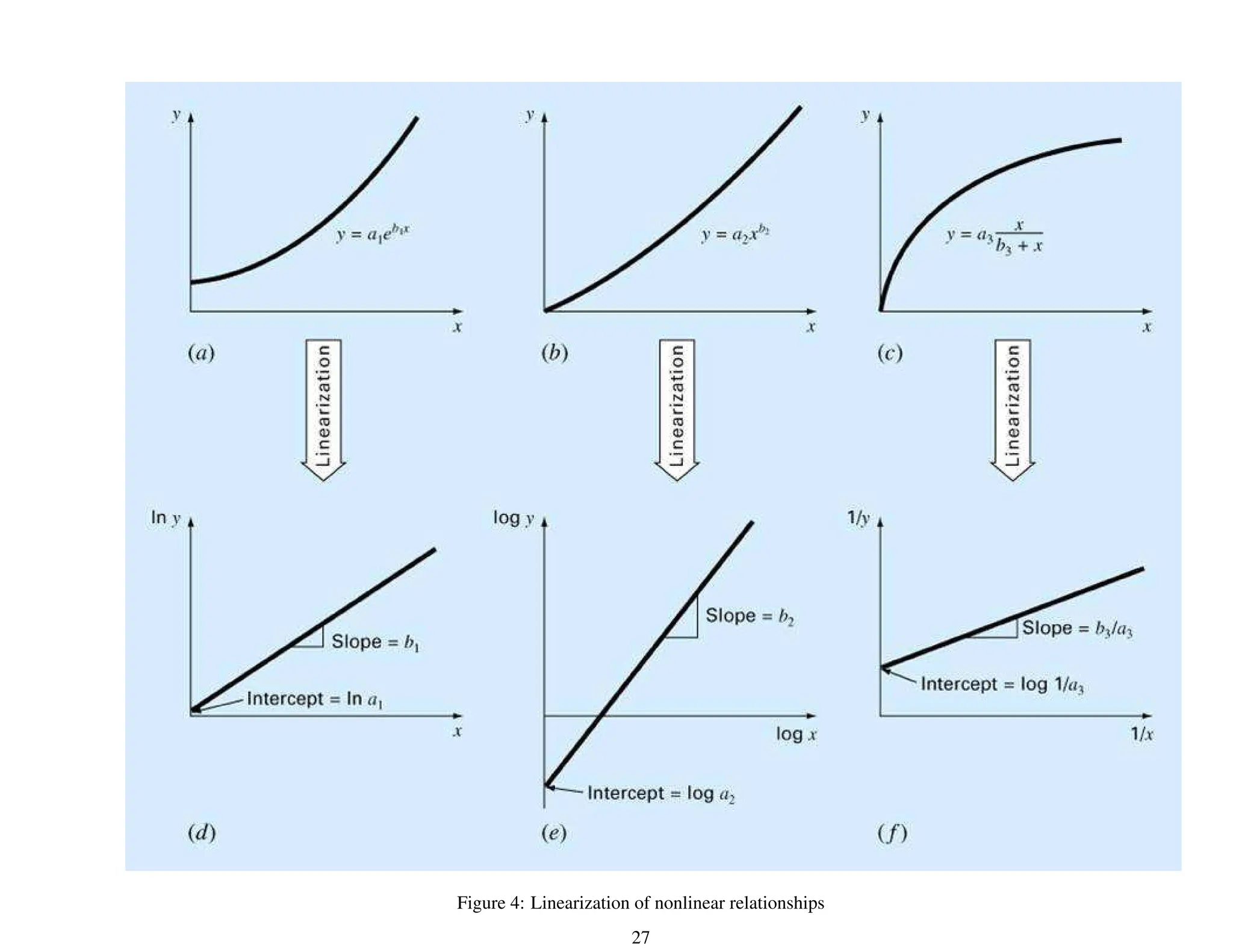
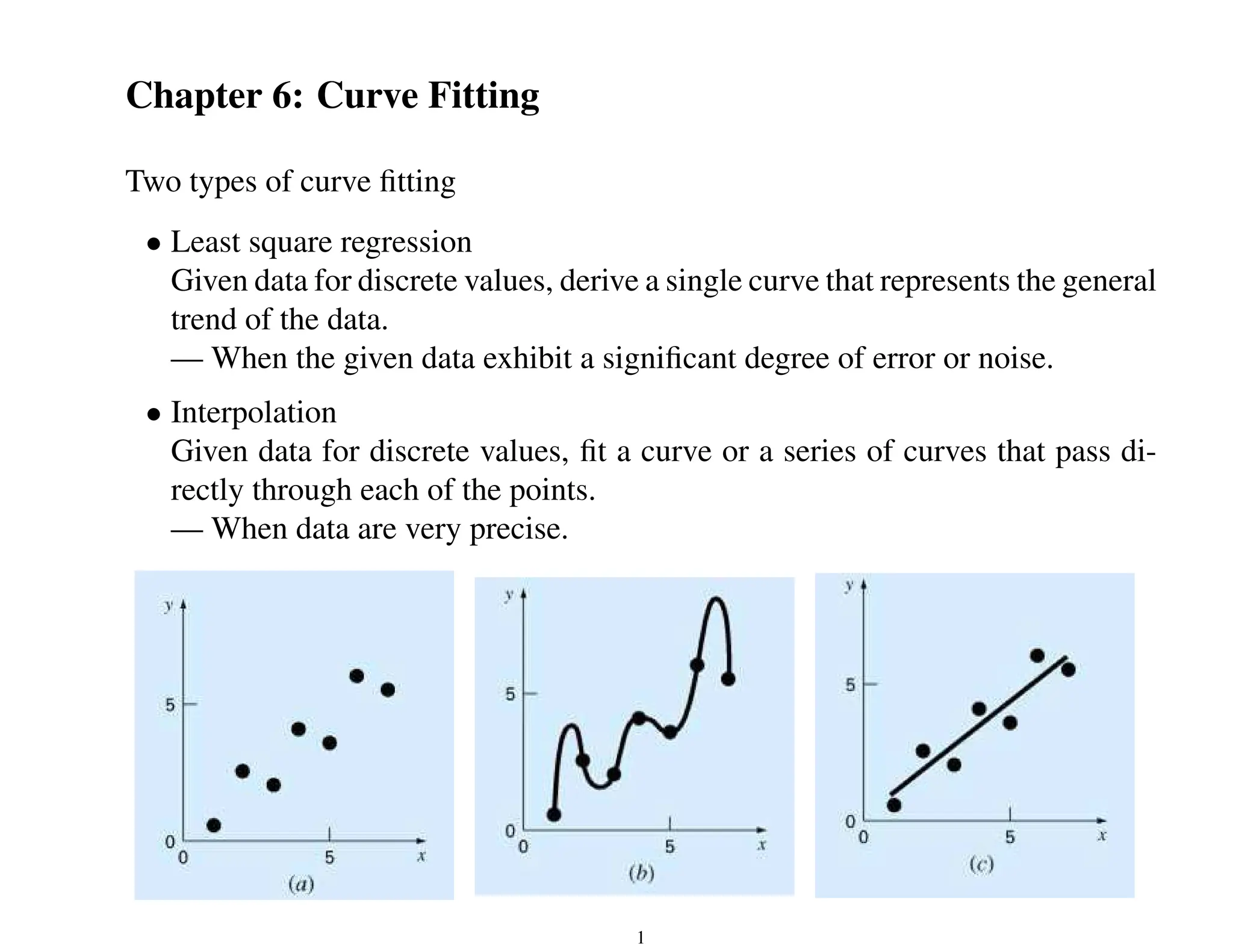
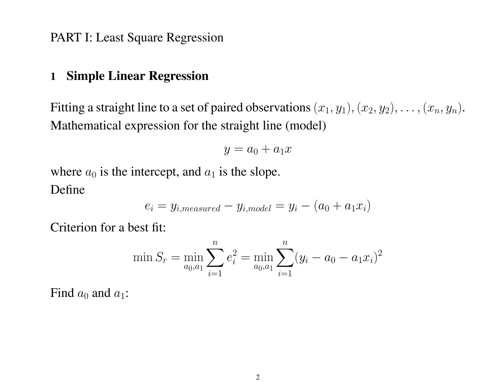
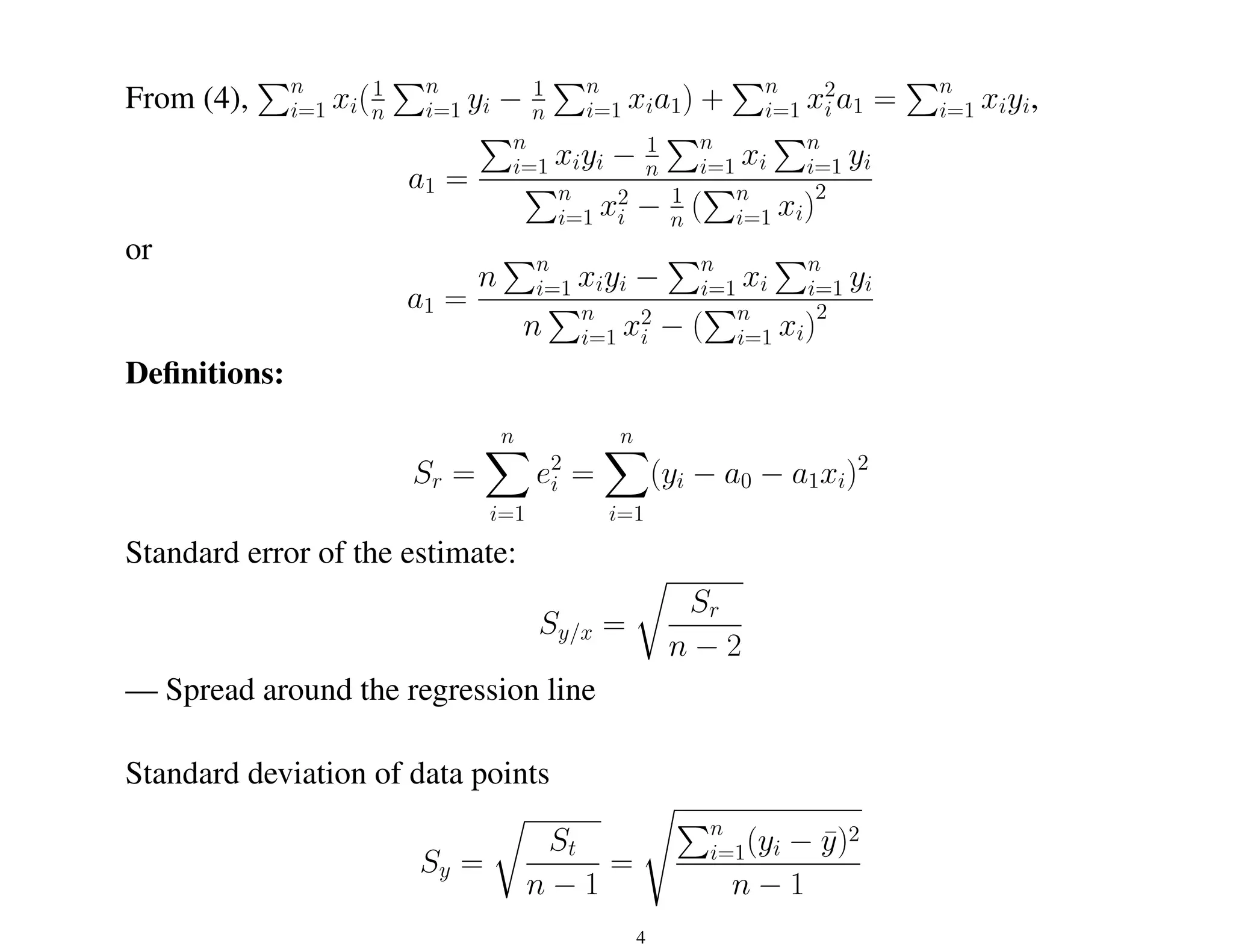
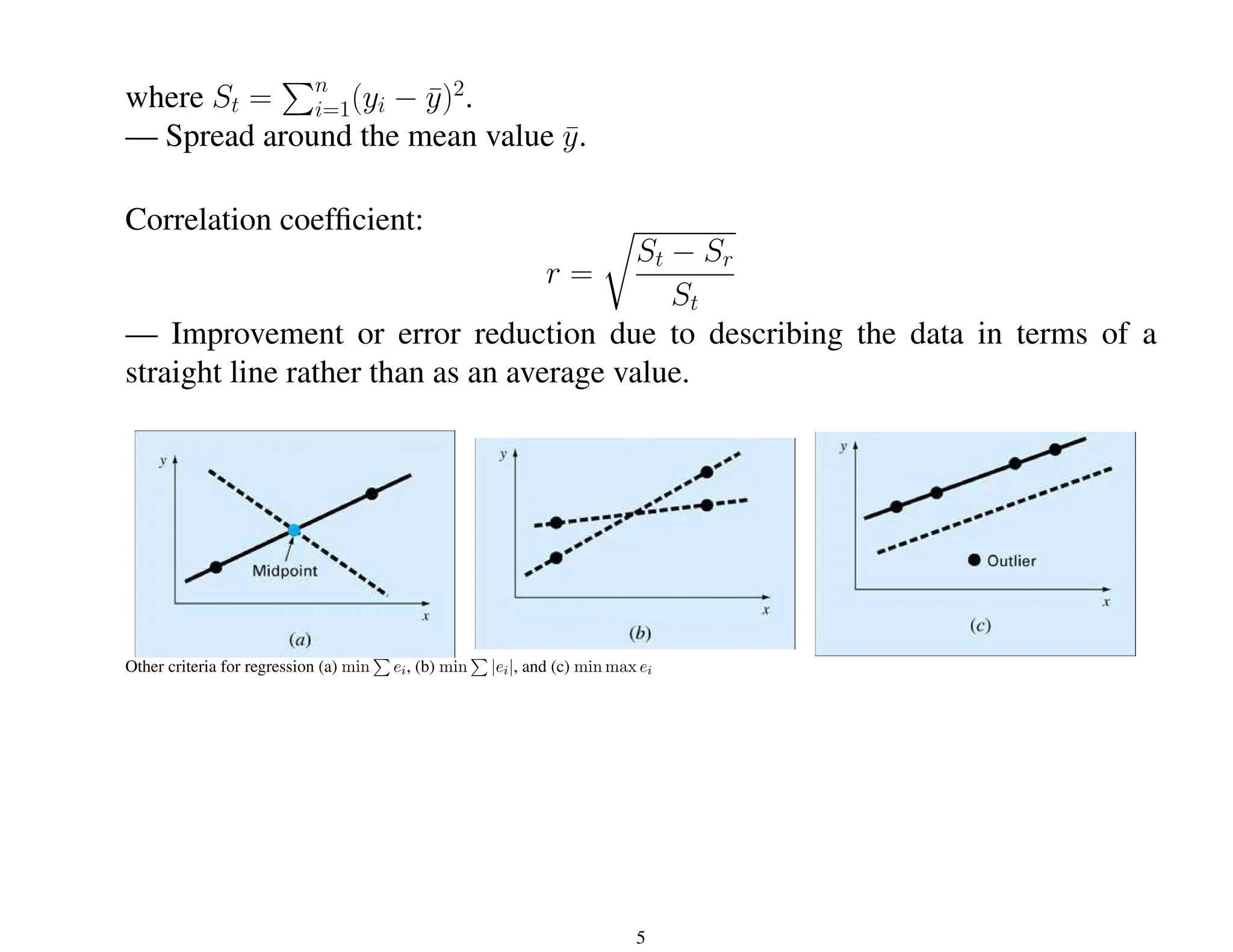
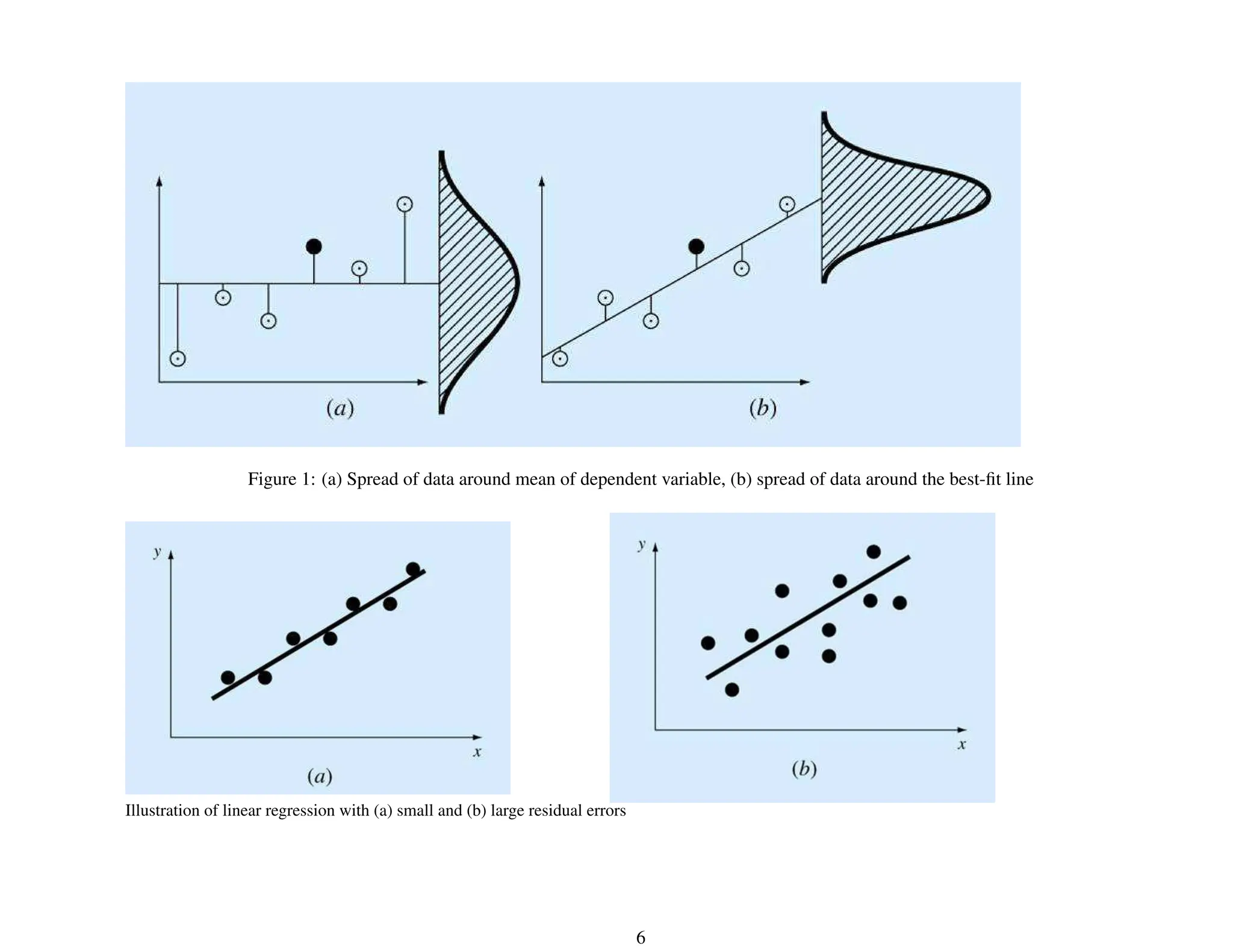
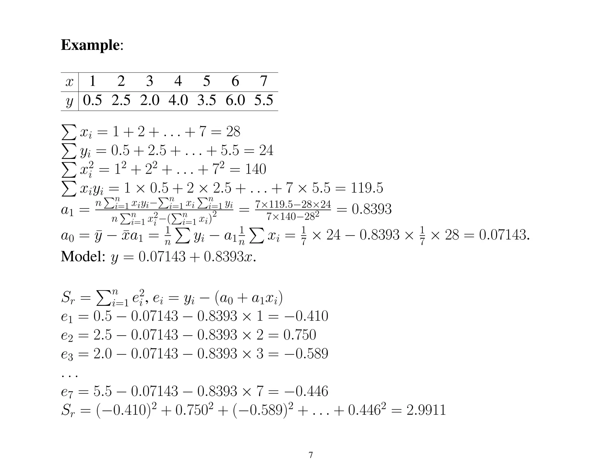
This document discusses techniques for curve fitting data, including least squares regression and interpolation. It covers: - Two types of curve fitting: least squares regression to derive a trend line for noisy data, and interpolation to fit curves passing through precise data points. - Linear regression to fit a straight line model and determine coefficients by minimizing the residual sum of squares. 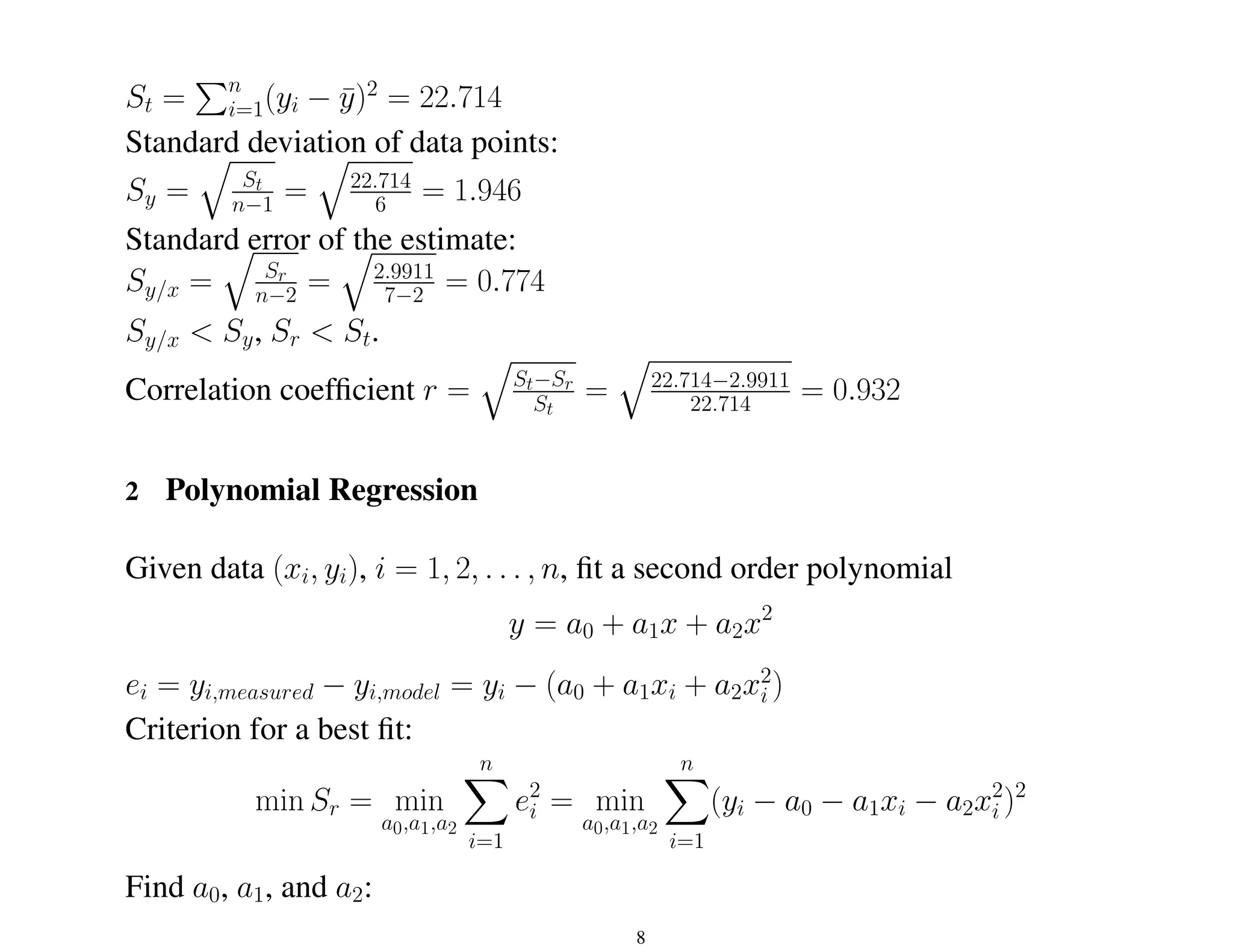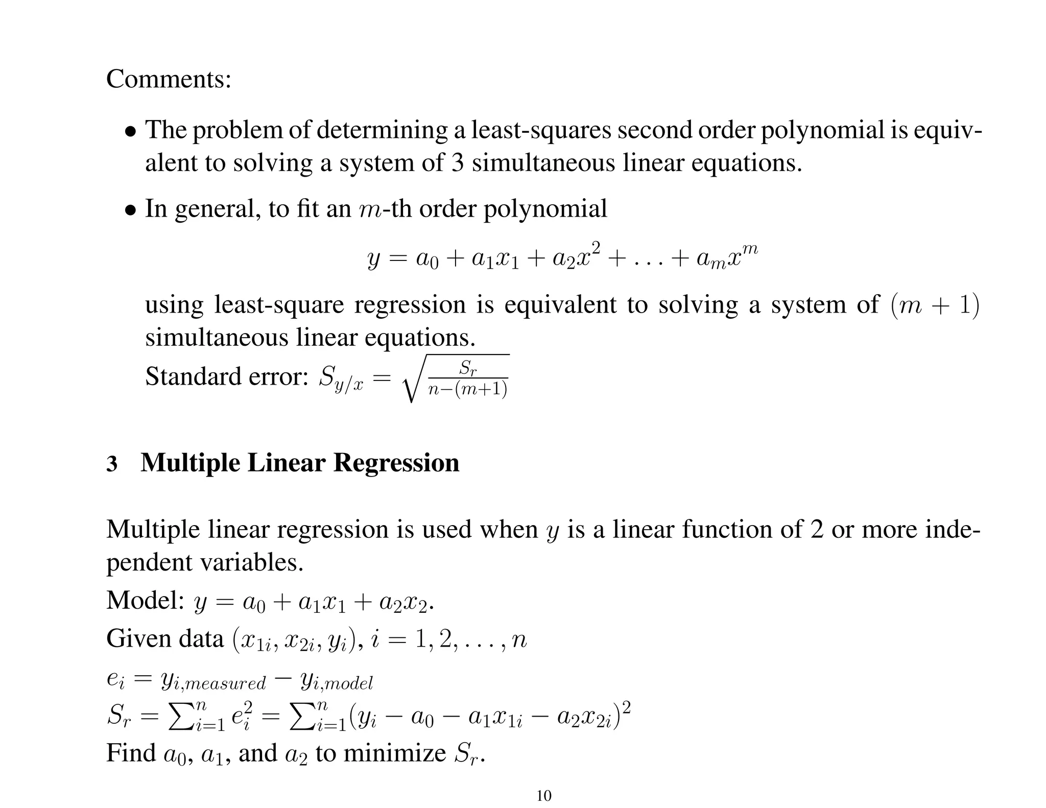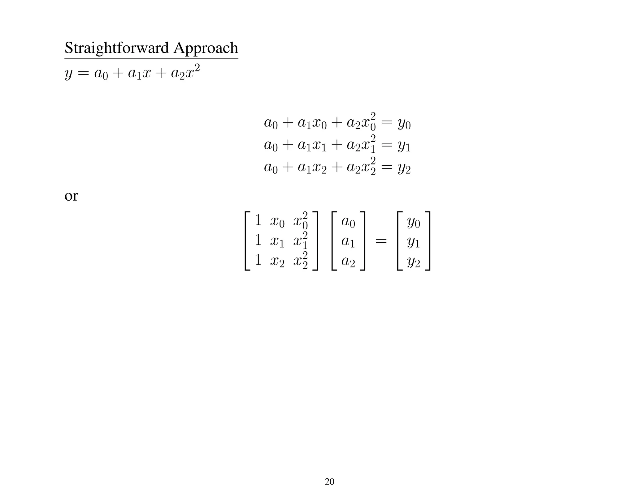- Polynomial regression to fit higher order polynomial models. 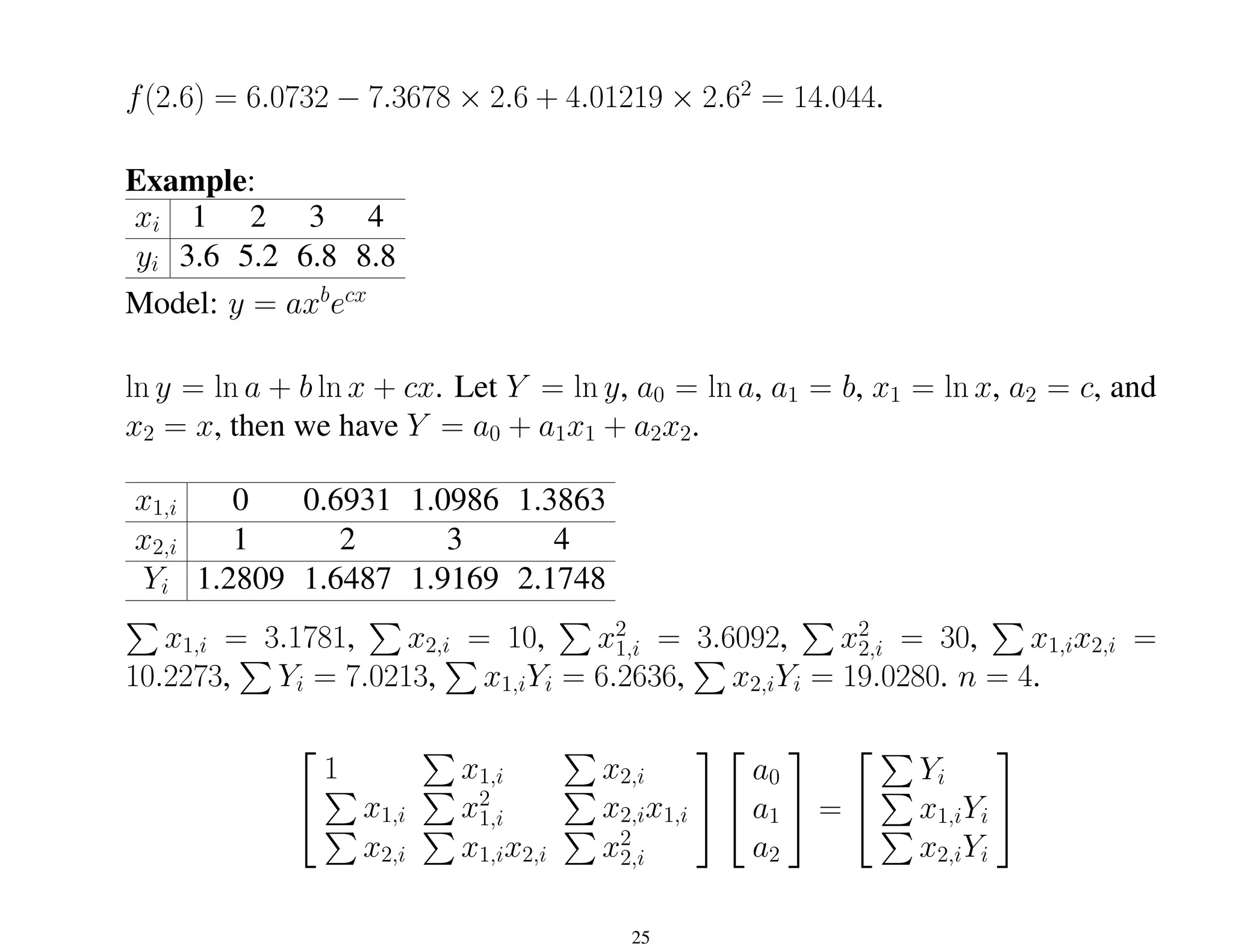- Multiple linear regression to fit models with multiple independent variables. 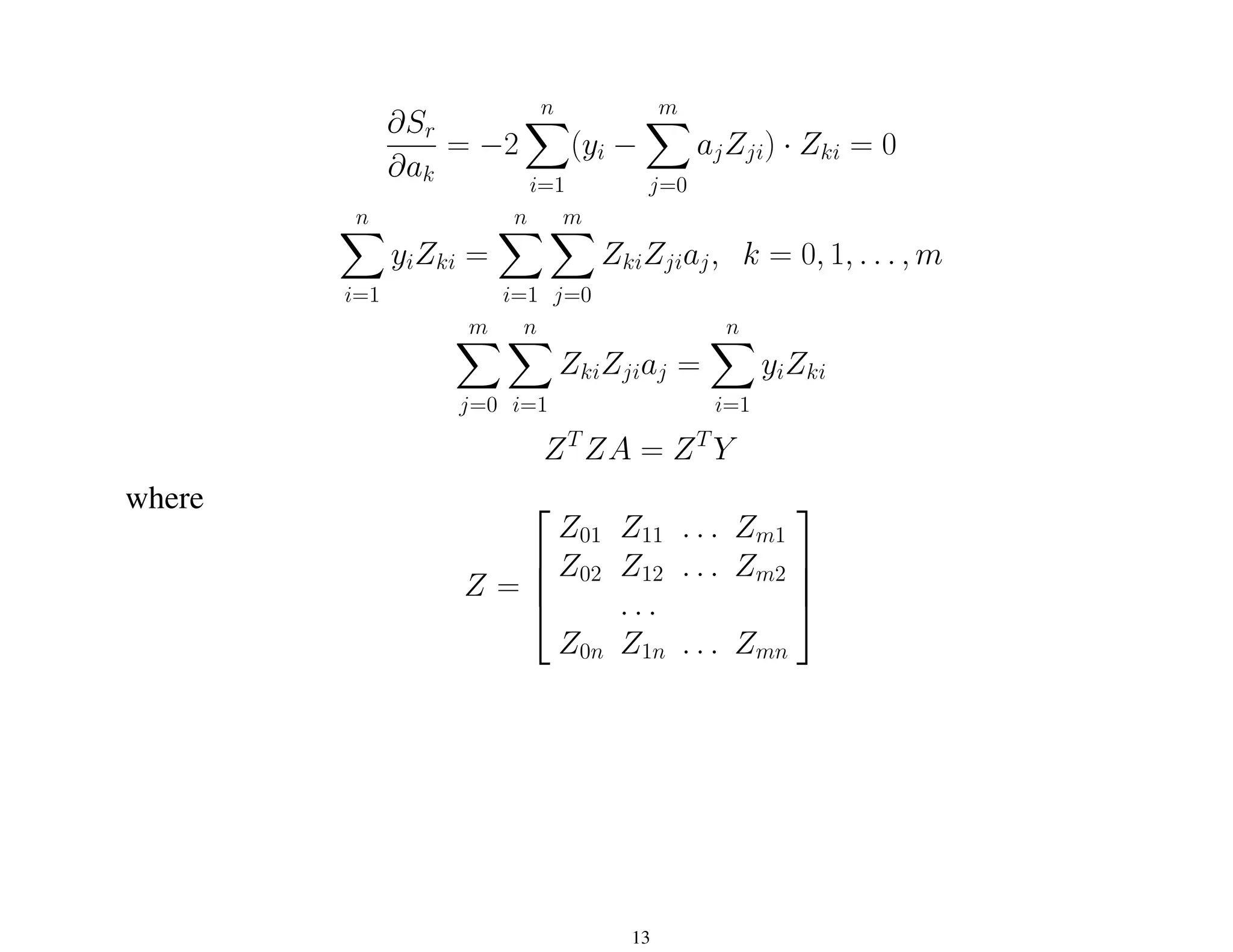- General linear least squares framework and normal equations to determine coefficients for any linear model. 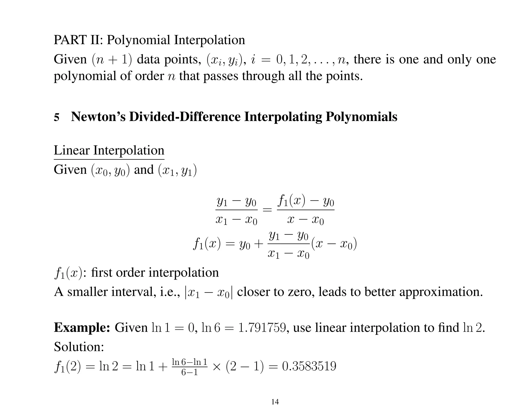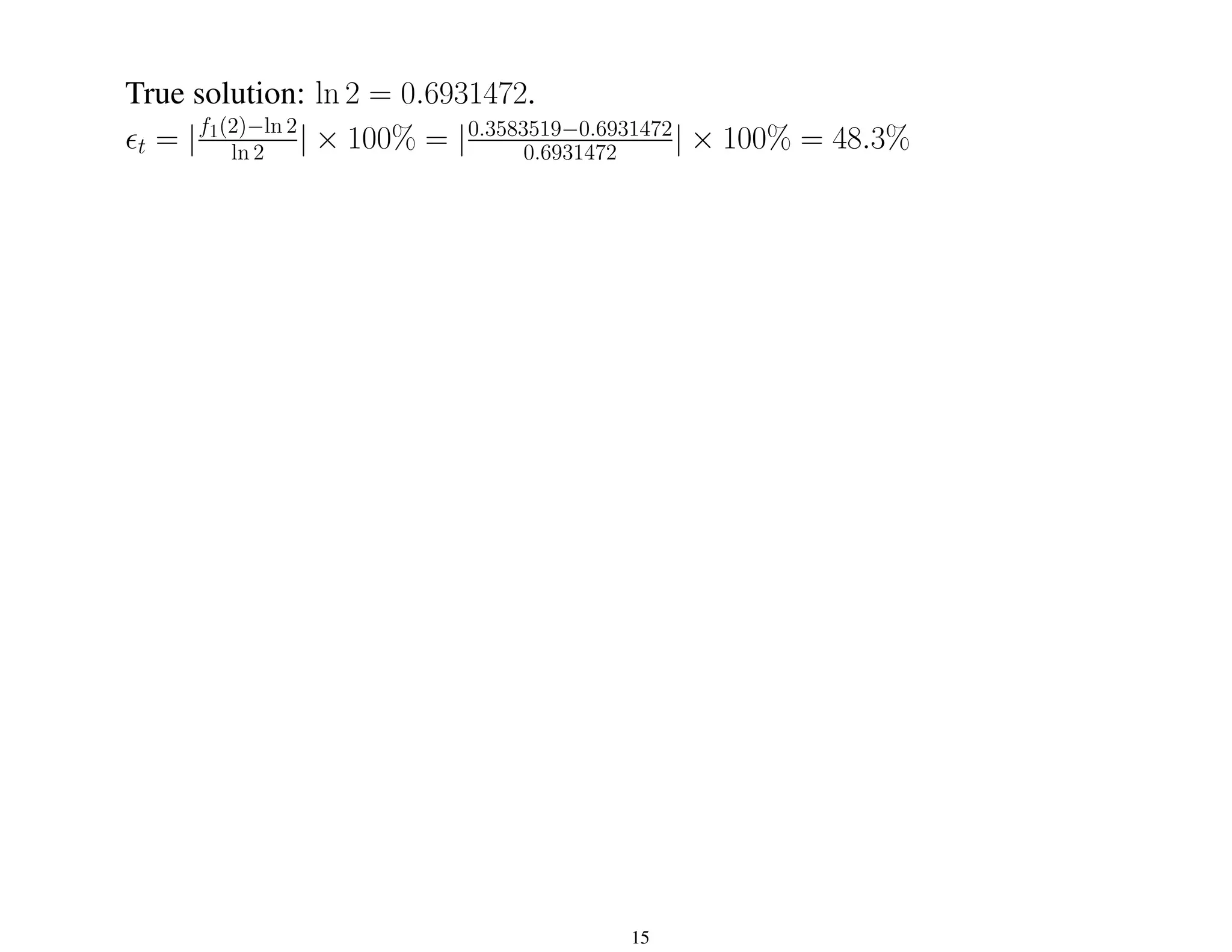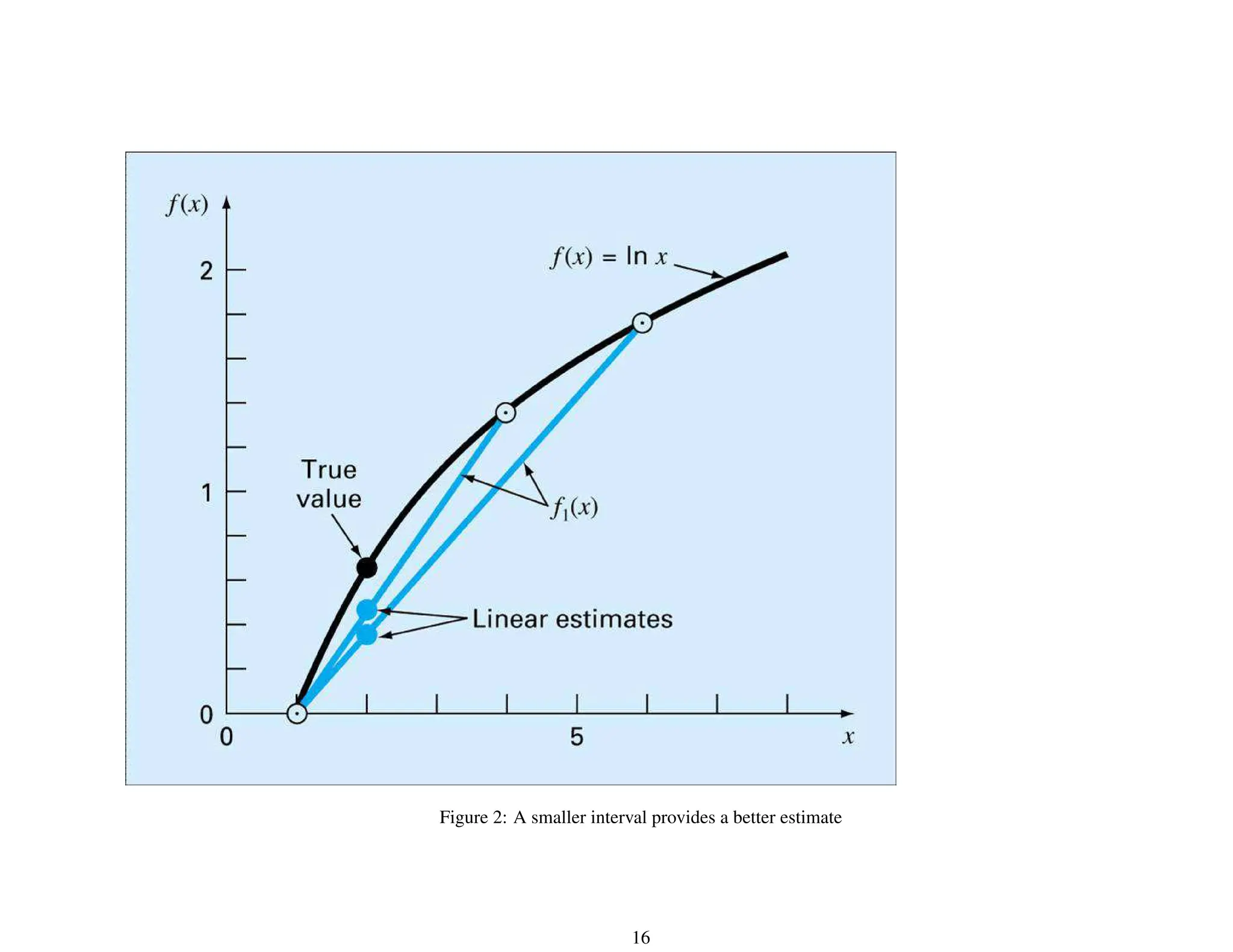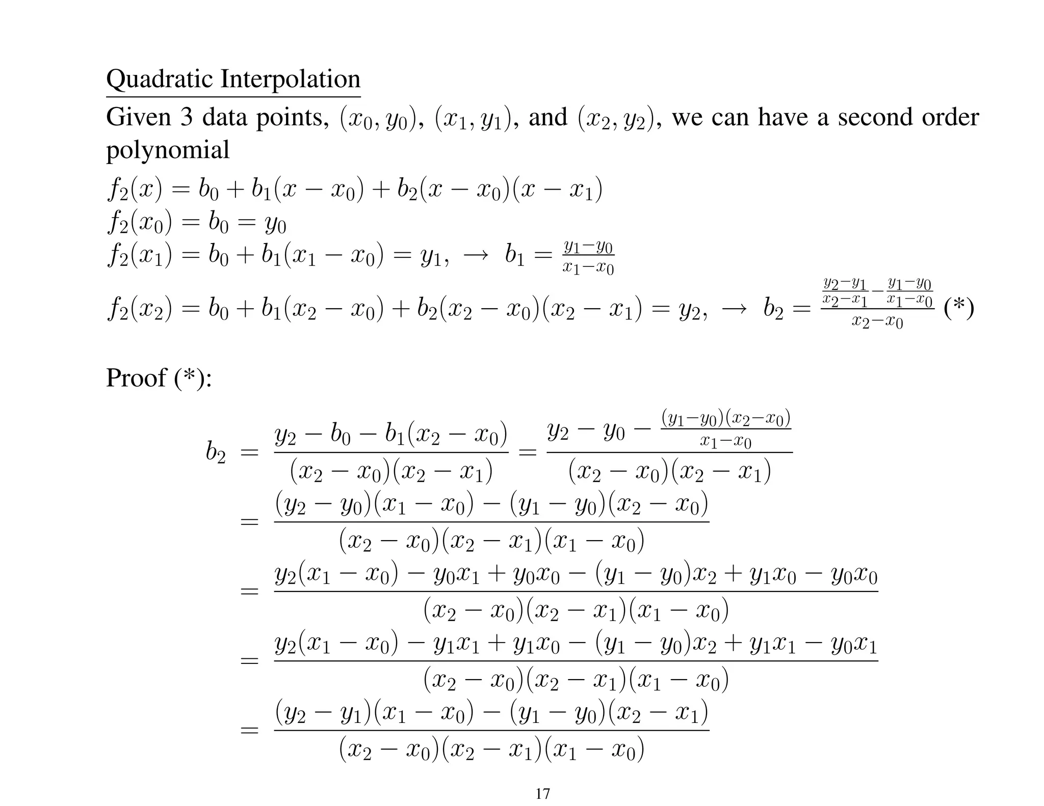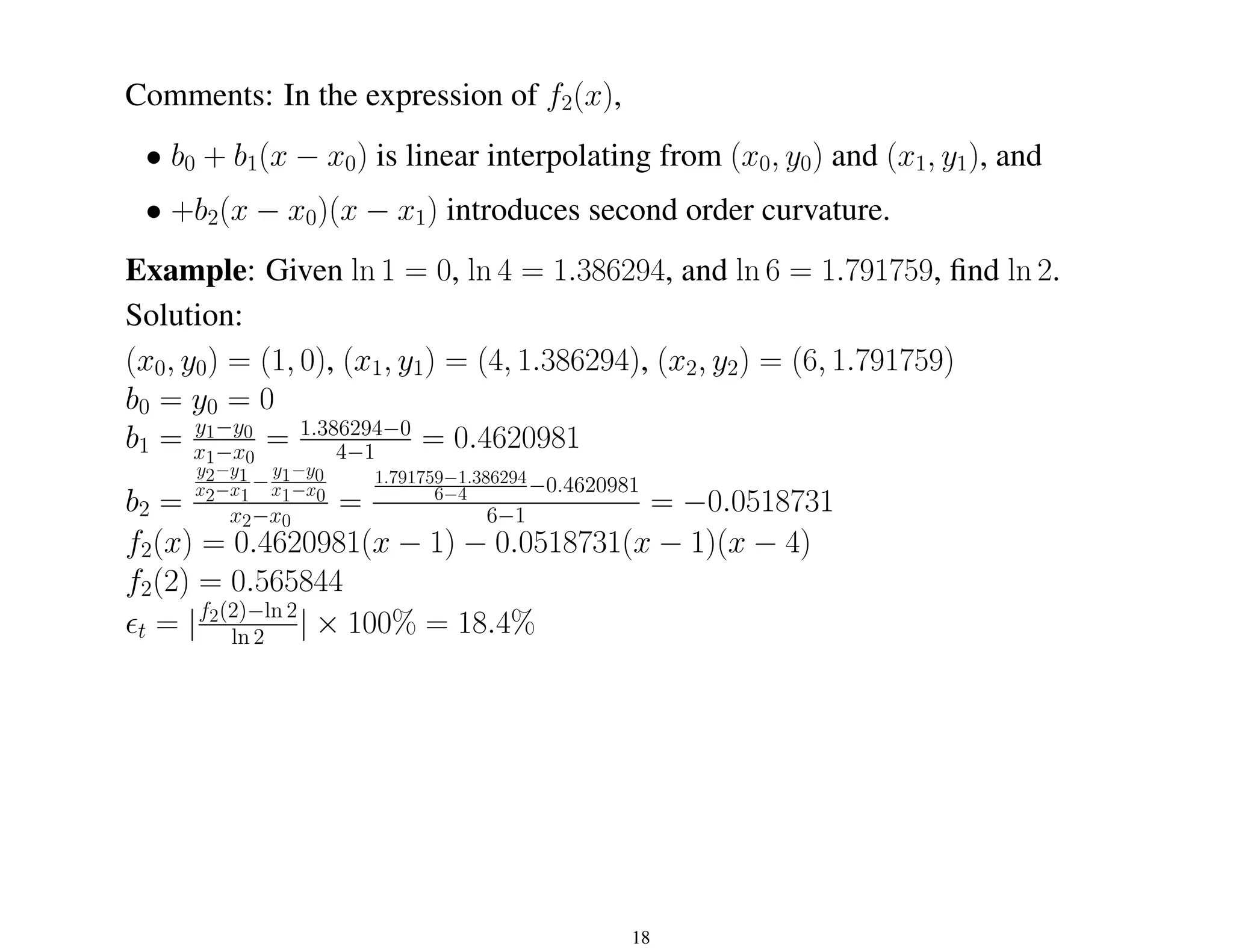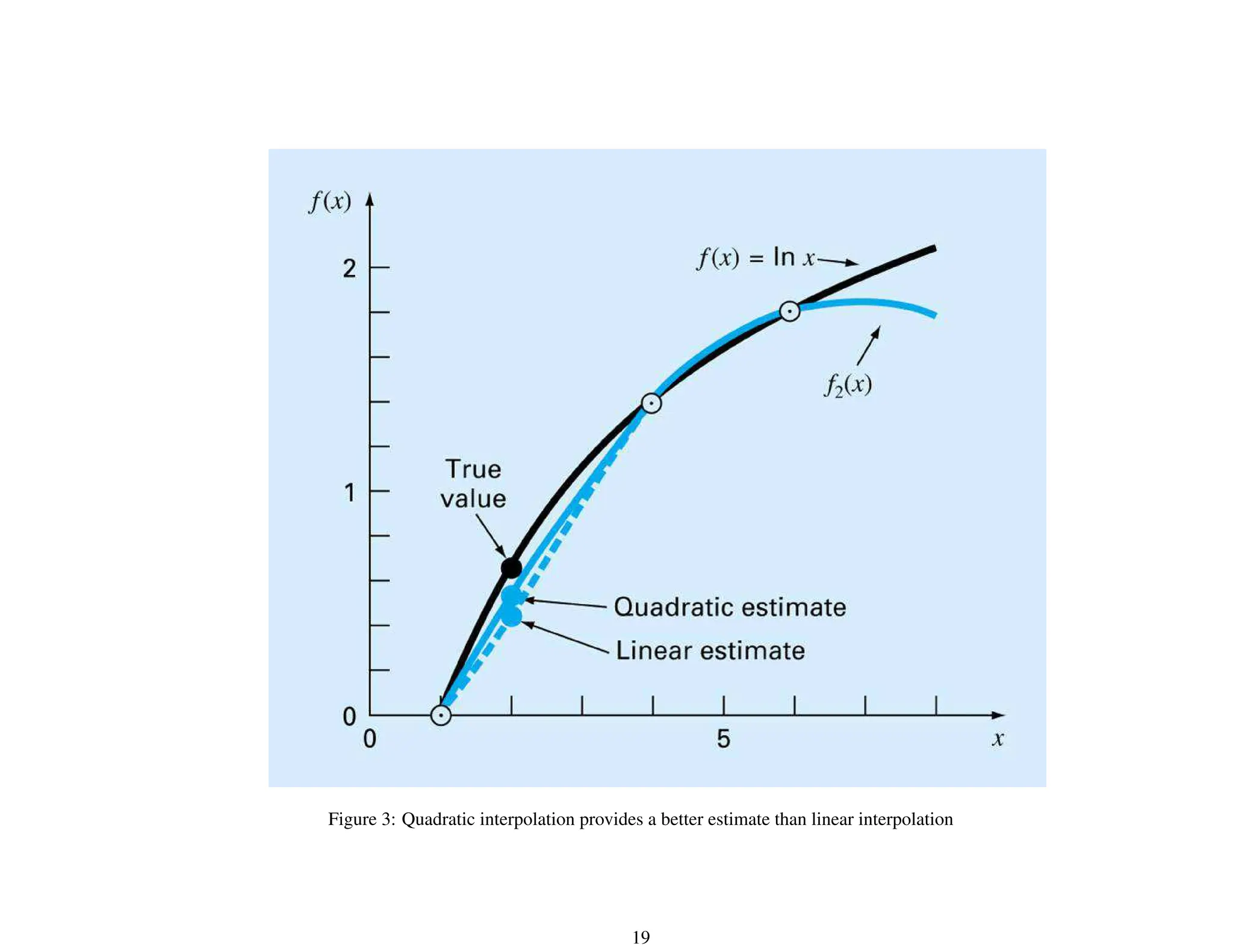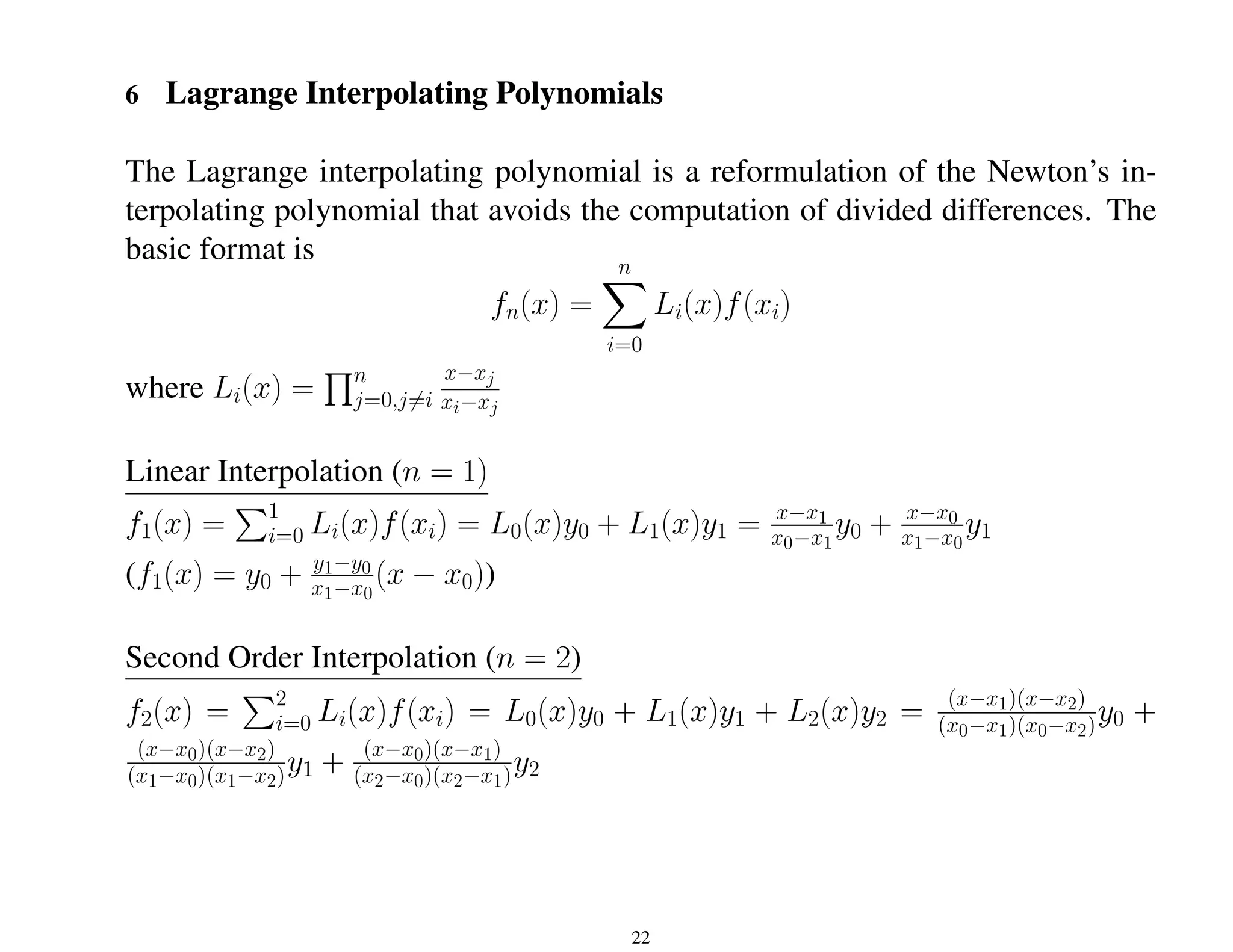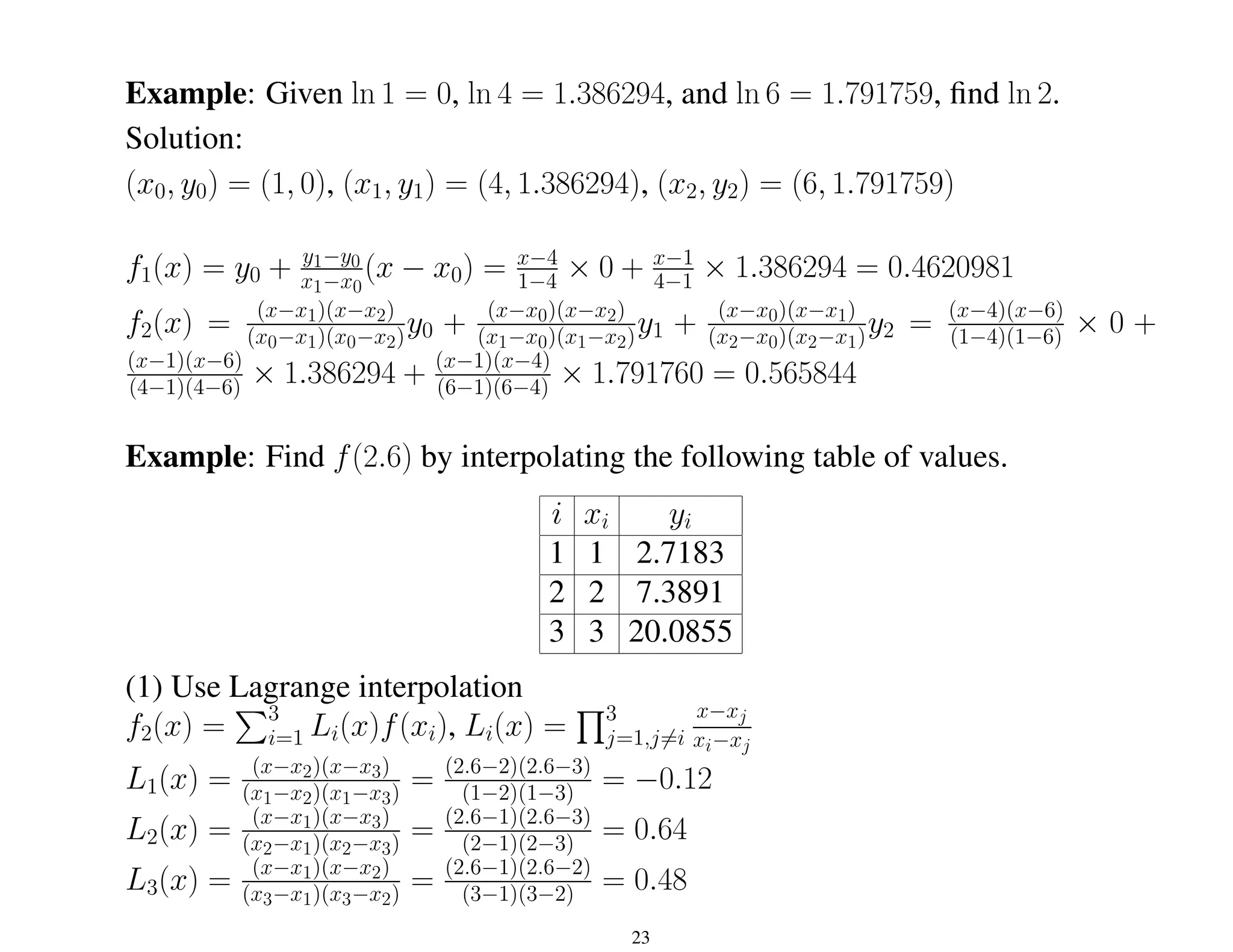- Polynomial interpolation to exactly fit curves through data points using divided differences.

1. Chapter 6: Curve Fitting
Two types of curve fitting
• Least square regression
Given data for discrete values, derive a single curve that represents the general
trend of the data.
— When the given data exhibit a significant degree of error or noise.
• Interpolation
Given data for discrete values, fit a curve or a series of curves that pass di-
rectly through each of the points.
— When data are very precise.
1

2. PART I: Least Square Regression
1 Simple Linear Regression
Fitting a straight line to a set of paired observations (x1, y1), (x2, y2), . . . , (xn, yn).
Mathematical expression for the straight line (model)
y = a0 + a1x
where a0 is the intercept, and a1 is the slope.
Define
ei = yi,measured − yi,model = yi − (a0 + a1xi)
Criterion for a best fit:
min Sr = min
a0,a1
n
X
i=1
e2
i = min
a0,a1
n
X
i=1
(yi − a0 − a1xi)2
Find a0 and a1:
2

3. ∂Sr
∂a0
= −2
n
X
i=1
(yi − a0 − a1xi) = 0 (1)
∂Sr
∂a1
= −2
n
X
i=1
[(yi − a0 − a1xi)xi] = 0 (2)
From (1),
Pn
i=1 yi −
Pn
i=1 a0 −
Pn
i=1 a1xi = 0, or
na0 +
n
X
i=1
xia1 =
n
X
i=1
yi (3)
From (2),
Pn
i=1 xiyi −
Pn
i=1 a0xi −
Pn
i=1 a1x2
i = 0, or
n
X
i=1
xia0 +
n
X
i=1
x2
i a1 =
n
X
i=1
xiyi (4)
(3) and (4) are called normal equations.
From (3),
a0 =
1
n
n
X
i=1
yi −
1
n
n
X
i=1
xia1 = ȳ − x̄a1
where x̄ = 1
n
Pn
i=1 xi, ȳ = 1
n
Pn
i=1 yi.
3

4. From (4),
Pn
i=1 xi(1
n
Pn
i=1 yi − 1
n
Pn
i=1 xia1) +
Pn
i=1 x2
i a1 =
Pn
i=1 xiyi,
a1 =
Pn
i=1 xiyi − 1
n
Pn
i=1 xi
Pn
i=1 yi
Pn
i=1 x2
i − 1
n (
Pn
i=1 xi)
2
or
a1 =
n
Pn
i=1 xiyi −
Pn
i=1 xi
Pn
i=1 yi
n
Pn
i=1 x2
i − (
Pn
i=1 xi)
2
Definitions:
Sr =
n
X
i=1
e2
i =
n
X
i=1
(yi − a0 − a1xi)2
Standard error of the estimate:
Sy/x =
r
Sr
n − 2
— Spread around the regression line
Standard deviation of data points
Sy =
r
St
n − 1
=
sPn
i=1(yi − ȳ)2
n − 1
4

5. where St =
Pn
i=1(yi − ȳ)2
.
— Spread around the mean value ȳ.
Correlation coefficient:
r =
r
St − Sr
St
— Improvement or error reduction due to describing the data in terms of a
straight line rather than as an average value.
Other criteria for regression (a) min
P
ei, (b) min
P
|ei|, and (c) min max ei
5

6. Figure 1: (a) Spread of data around mean of dependent variable, (b) spread of data around the best-fit line
Illustration of linear regression with (a) small and (b) large residual errors
6

7. Example:
x 1 2 3 4 5 6 7
y 0.5 2.5 2.0 4.0 3.5 6.0 5.5
P
xi = 1 + 2 + . . . + 7 = 28
P
yi = 0.5 + 2.5 + . . . + 5.5 = 24
P
x2
i = 12
+ 22
+ . . . + 72
= 140
P
xiyi = 1 × 0.5 + 2 × 2.5 + . . . + 7 × 5.5 = 119.5
a1 =
n
Pn
i=1 xiyi−
Pn
i=1 xi
Pn
i=1 yi
n
Pn
i=1 x2
i −(
Pn
i=1 xi)2 = 7×119.5−28×24
7×140−282 = 0.8393
a0 = ȳ − x̄a1 = 1
n
P
yi − a1
1
n
P
xi = 1
7 × 24 − 0.8393 × 1
7 × 28 = 0.07143.
Model: y = 0.07143 + 0.8393x.
Sr =
Pn
i=1 e2
i , ei = yi − (a0 + a1xi)
e1 = 0.5 − 0.07143 − 0.8393 × 1 = −0.410
e2 = 2.5 − 0.07143 − 0.8393 × 2 = 0.750
e3 = 2.0 − 0.07143 − 0.8393 × 3 = −0.589
. . .
e7 = 5.5 − 0.07143 − 0.8393 × 7 = −0.446
Sr = (−0.410)2
+ 0.7502
+ (−0.589)2
+ . . . + 0.4462
= 2.9911
7

8. St =
Pn
i=1(yi − ȳ)2
= 22.714
Standard deviation of data points:
Sy =
q
St
n−1 =
q
22.714
6 = 1.946
Standard error of the estimate:
Sy/x =
q
Sr
n−2 =
q
2.9911
7−2 = 0.774
Sy/x < Sy, Sr < St.
Correlation coefficient r =
q
St−Sr
St
=
q
22.714−2.9911
22.714 = 0.932
2 Polynomial Regression
Given data (xi, yi), i = 1, 2, . . . , n, fit a second order polynomial
y = a0 + a1x + a2x2
ei = yi,measured − yi,model = yi − (a0 + a1xi + a2x2
i )
Criterion for a best fit:
min Sr = min
a0,a1,a2
n
X
i=1
e2
i = min
a0,a1,a2
n
X
i=1
(yi − a0 − a1xi − a2x2
i )2
Find a0, a1, and a2:
8

9. ∂Sr
∂a0
= −2
n
X
i=1
(yi − a0 − a1xi − a2x2
i ) = 0 (1)
∂Sr
∂a1
= −2
n
X
i=1
[(yi − a0 − a1xi − a2x2
i )xi] = 0 (2)
∂Sr
∂a2
= −2
n
X
i=1
[(yi − a0 − a1xi − a2x2
i )x2
i ] = 0 (3)
From (1),
Pn
i=1 yi −
Pn
i=1 a0 −
Pn
i=1 a1xi −
Pn
i=1 a2x2
i = 0, or
na0 +
n
X
i=1
xia1 +
n
X
i=1
x2
i a2 =
n
X
i=1
yi (1
0
)
From (2),
Pn
i=1 xiyi −
Pn
i=1 a0xi −
Pn
i=1 a1x2
i −
Pn
i=1 x3
i a2 = 0, or
n
X
i=1
xia0 +
n
X
i=1
x2
i a1 +
n
X
i=1
x3
i a2 =
n
X
i=1
xiyi (2
0
)
From (3),
Pn
i=1 x2
i yi −
Pn
i=1 a0x2
i −
Pn
i=1 a1x3
i −
Pn
i=1 x4
i a2 = 0, or
n
X
i=1
x2
i a0 +
n
X
i=1
x3
i a1 +
n
X
i=1
x4
i a2 =
n
X
i=1
x2
i yi (3
0
)
9

10. Comments:
• The problem of determining a least-squares second order polynomial is equiv-
alent to solving a system of 3 simultaneous linear equations.
• In general, to fit an m-th order polynomial
y = a0 + a1x1 + a2x2
+ . . . + amxm
using least-square regression is equivalent to solving a system of (m + 1)
simultaneous linear equations.
Standard error: Sy/x =
q
Sr
n−(m+1)
3 Multiple Linear Regression
Multiple linear regression is used when y is a linear function of 2 or more inde-
pendent variables.
Model: y = a0 + a1x1 + a2x2.
Given data (x1i, x2i, yi), i = 1, 2, . . . , n
ei = yi,measured − yi,model
Sr =
Pn
i=1 e2
i =
Pn
i=1(yi − a0 − a1x1i − a2x2i)2
Find a0, a1, and a2 to minimize Sr.
10

11. ∂Sr
∂a0
= −2
n
X
i=1
(yi − a0 − a1x1i − a2x2i) = 0 (1)
∂Sr
∂a1
= −2
n
X
i=1
[(yi − a0 − a1x1i − a2x2i)x1i] = 0 (2)
∂Sr
∂a2
= −2
n
X
i=1
[(yi − a0 − a1x1i − a2x2i)x2i] = 0 (3)
From (1), na0 +
Pn
i=1 x1ia1 +
Pn
i=1 x2ia2 =
Pn
i=1 yi (1
0
)
From (2),
Pn
i=1 x1ia0 +
Pn
i=1 x2
1ia1 +
Pn
i=1 x1ix2ia2 =
Pn
i=1 x1iyi (2
0
)
From (3),
Pn
i=1 x2ia0 +
Pn
i=1 x1ix2ia1 +
Pn
i=1 x2
2ia2 =
Pn
i=1 x2iyi (3
0
)


n
P
x1i
P
x2i
P
x1i
P
x2
1i
P
x1ix2i
P
x2i
P
x1ix2i
P
x2
2i




a0
a1
a2

 =


P
yi
P
x1iyi
P
x2iyi


Standard error: Sy/x =
q
Sr
n−(m+1)
11

12. 4 General Linear Least Squares
Model:
y = a0Z0 + a1Z1 + a2Z2 + . . . + amZm
where Z0, Z1, . . . , Zm are (m + 1) different functions.
Special cases:
• Simple linear LSR: Z0 = 1, Z1 = x, Zi = 0 for i ≥ 2
• Polynomial LSR: Zi = xi
(Z0 = 1, Z1 = x, Z2 = x2
, ...)
• Multiple linear LSR: Z0 = 1, Zi = xi for i ≥ 1
“Linear” indicates the model’s dependence on its parameters, ai’s. The functions
can be highly non-linear.
Sr =
Pn
i=1 e2
i =
Pn
i=1(yi,measured − yi,model)2
Given data (Z0i, Z1i, . . . , Zmi, yi), i = 1, 2, . . . , n,
Sr =
n
X
i=1
(yi −
m
X
j=0
ajZji)2
Find aj, j = 0, 1, 2, . . . , m to minimize Sr.
12

13. ∂Sr
∂ak
= −2
n
X
i=1
(yi −
m
X
j=0
ajZji) · Zki = 0
n
X
i=1
yiZki =
n
X
i=1
m
X
j=0
ZkiZjiaj, k = 0, 1, . . . , m
m
X
j=0
n
X
i=1
ZkiZjiaj =
n
X
i=1
yiZki
ZT
ZA = ZT
Y
where
Z =




Z01 Z11 . . . Zm1
Z02 Z12 . . . Zm2
. . .
Z0n Z1n . . . Zmn




13

14. PART II: Polynomial Interpolation
Given (n + 1) data points, (xi, yi), i = 0, 1, 2, . . . , n, there is one and only one
polynomial of order n that passes through all the points.
5 Newton’s Divided-Difference Interpolating Polynomials
Linear Interpolation
Given (x0, y0) and (x1, y1)
y1 − y0
x1 − x0
=
f1(x) − y0
x − x0
f1(x) = y0 +
y1 − y0
x1 − x0
(x − x0)
f1(x): first order interpolation
A smaller interval, i.e., |x1 − x0| closer to zero, leads to better approximation.
Example: Given ln 1 = 0, ln 6 = 1.791759, use linear interpolation to find ln 2.
Solution:
f1(2) = ln 2 = ln 1 + ln 6−ln 1
6−1 × (2 − 1) = 0.3583519
14

15. True solution: ln 2 = 0.6931472.
²t = |f1(2)−ln 2
ln 2 | × 100% = |0.3583519−0.6931472
0.6931472 | × 100% = 48.3%
15

16. Figure 2: A smaller interval provides a better estimate
16

17. Quadratic Interpolation
Given 3 data points, (x0, y0), (x1, y1), and (x2, y2), we can have a second order
polynomial
f2(x) = b0 + b1(x − x0) + b2(x − x0)(x − x1)
f2(x0) = b0 = y0
f2(x1) = b0 + b1(x1 − x0) = y1, → b1 = y1−y0
x1−x0
f2(x2) = b0 + b1(x2 − x0) + b2(x2 − x0)(x2 − x1) = y2, → b2 =
y2−y1
x2−x1
−
y1−y0
x1−x0
x2−x0
(*)
Proof (*):
b2 =
y2 − b0 − b1(x2 − x0)
(x2 − x0)(x2 − x1)
=
y2 − y0 − (y1−y0)(x2−x0)
x1−x0
(x2 − x0)(x2 − x1)
=
(y2 − y0)(x1 − x0) − (y1 − y0)(x2 − x0)
(x2 − x0)(x2 − x1)(x1 − x0)
=
y2(x1 − x0) − y0x1 + y0x0 − (y1 − y0)x2 + y1x0 − y0x0
(x2 − x0)(x2 − x1)(x1 − x0)
=
y2(x1 − x0) − y1x1 + y1x0 − (y1 − y0)x2 + y1x1 − y0x1
(x2 − x0)(x2 − x1)(x1 − x0)
=
(y2 − y1)(x1 − x0) − (y1 − y0)(x2 − x1)
(x2 − x0)(x2 − x1)(x1 − x0)
17

18. Comments: In the expression of f2(x),
• b0 + b1(x − x0) is linear interpolating from (x0, y0) and (x1, y1), and
• +b2(x − x0)(x − x1) introduces second order curvature.
Example: Given ln 1 = 0, ln 4 = 1.386294, and ln 6 = 1.791759, find ln 2.
Solution:
(x0, y0) = (1, 0), (x1, y1) = (4, 1.386294), (x2, y2) = (6, 1.791759)
b0 = y0 = 0
b1 = y1−y0
x1−x0
= 1.386294−0
4−1 = 0.4620981
b2 =
y2−y1
x2−x1
−
y1−y0
x1−x0
x2−x0
=
1.791759−1.386294
6−4 −0.4620981
6−1 = −0.0518731
f2(x) = 0.4620981(x − 1) − 0.0518731(x − 1)(x − 4)
f2(2) = 0.565844
²t = |f2(2)−ln 2
ln 2 | × 100% = 18.4%
18

19. Figure 3: Quadratic interpolation provides a better estimate than linear interpolation
19

20. Straightforward Approach
y = a0 + a1x + a2x2
a0 + a1x0 + a2x2
0 = y0
a0 + a1x1 + a2x2
1 = y1
a0 + a1x2 + a2x2
2 = y2
or


1 x0 x2
0
1 x1 x2
1
1 x2 x2
2




a0
a1
a2

 =


y0
y1
y2


20

21. General Form of Newton’s Interpolating Polynomial
Given (n + 1) data points, (xi, yi), i = 0, 1, . . . , n, fit an n-th order polynomial
fn(x) = b0 +b1(x−x0)+. . .+bn(x−x0)(x−x1) . . . (x−xn) =
n
X
i=0
bi
i−1
Y
j=0
(x−xj)
find b0, b1, . . . , bn.
x = x0, y0 = b0 or b0 = y0.
x = x1, y1 = b0 + b1(x1 − x0), then b1 = y1−y0
x1−x0
Define b1 = f[x1, x0] = y1−y0
x1−x0
.
x = x2, y2 = b0 + b1(x2 − x0) + b2(x2 − x0)(x2 − x1), then b2 =
y2−y1
x2−x1
−
y1−y0
x1−x0
x2−x0
Define f[x2, x1, x0] = f[x2,x1]−f[x1,x0]
x2−x0
, then b2 = f[x2, x1, x0].
. . .
x = xn, bn = f[xn, xn−1, . . . , x1, x0] = f[xn,xn−1,...,x1]−f[xn−1,...,x1,x0]
xn−x0
21

22. 6 Lagrange Interpolating Polynomials
The Lagrange interpolating polynomial is a reformulation of the Newton’s in-
terpolating polynomial that avoids the computation of divided differences. The
basic format is
fn(x) =
n
X
i=0
Li(x)f(xi)
where Li(x) =
Qn
j=0,j6=i
x−xj
xi−xj
Linear Interpolation (n = 1)
f1(x) =
P1
i=0 Li(x)f(xi) = L0(x)y0 + L1(x)y1 = x−x1
x0−x1
y0 + x−x0
x1−x0
y1
(f1(x) = y0 + y1−y0
x1−x0
(x − x0))
Second Order Interpolation (n = 2)
f2(x) =
P2
i=0 Li(x)f(xi) = L0(x)y0 + L1(x)y1 + L2(x)y2 = (x−x1)(x−x2)
(x0−x1)(x0−x2)y0 +
(x−x0)(x−x2)
(x1−x0)(x1−x2)y1 + (x−x0)(x−x1)
(x2−x0)(x2−x1)y2
22

23. Example: Given ln 1 = 0, ln 4 = 1.386294, and ln 6 = 1.791759, find ln 2.
Solution:
(x0, y0) = (1, 0), (x1, y1) = (4, 1.386294), (x2, y2) = (6, 1.791759)
f1(x) = y0 + y1−y0
x1−x0
(x − x0) = x−4
1−4 × 0 + x−1
4−1 × 1.386294 = 0.4620981
f2(x) = (x−x1)(x−x2)
(x0−x1)(x0−x2)y0 + (x−x0)(x−x2)
(x1−x0)(x1−x2)y1 + (x−x0)(x−x1)
(x2−x0)(x2−x1)y2 = (x−4)(x−6)
(1−4)(1−6) × 0 +
(x−1)(x−6)
(4−1)(4−6) × 1.386294 + (x−1)(x−4)
(6−1)(6−4) × 1.791760 = 0.565844
Example: Find f(2.6) by interpolating the following table of values.
i xi yi
1 1 2.7183
2 2 7.3891
3 3 20.0855
(1) Use Lagrange interpolation
f2(x) =
P3
i=1 Li(x)f(xi), Li(x) =
Q3
j=1,j6=i
x−xj
xi−xj
L1(x) = (x−x2)(x−x3)
(x1−x2)(x1−x3) = (2.6−2)(2.6−3)
(1−2)(1−3) = −0.12
L2(x) = (x−x1)(x−x3)
(x2−x1)(x2−x3) = (2.6−1)(2.6−3)
(2−1)(2−3) = 0.64
L3(x) = (x−x1)(x−x2)
(x3−x1)(x3−x2) = (2.6−1)(2.6−2)
(3−1)(3−2) = 0.48
23

24. f2(2.6) = −0.12 × 2.7183 + 0.64 × 7.3891 + 0.48 × 20.08853 = 14.0439
(2) use Newton’s interpolation
f2(x) = b0 + b1(x − x1) + b2(x − x1)(x − x2)
b0 = y1 = 2.7183
b1 = y2−y1
x2−x1
= 7.3891−2.7183
2−1 = 4.6708
b2 =
y2−y1
x2−x1
−
y1−y0
x1−x0
x2−x0
=
20.0855−7.3891
3−2 −4.6708
3−1 = 4.0128
f2(2.6) = 2.7183 + 4.6708 × (2.6 − 1) + 4.0128 × (2.6 − 1)(2.6 − 2) = 14.0439
(3) Use the straightforward method
f2(x) = a0 + a1x + a2x2
a0 + a1 + a2 × 12
= 2.7183
a0 + a1 + a2 × 22
= 7.3891
a0 + a1 + a2 × 32
= 20.0855
or 

1 1 1
1 2 4
1 3 9




a0
a1
a2

 =


2.7183
7.3891
20.0855


[a0 a1 a2]
0
= [6.0732; −7.3678 4.0129]
0
24

25. f(2.6) = 6.0732 − 7.3678 × 2.6 + 4.01219 × 2.62
= 14.044.
Example:
xi 1 2 3 4
yi 3.6 5.2 6.8 8.8
Model: y = axb
ecx
ln y = ln a + b ln x + cx. Let Y = ln y, a0 = ln a, a1 = b, x1 = ln x, a2 = c, and
x2 = x, then we have Y = a0 + a1x1 + a2x2.
x1,i 0 0.6931 1.0986 1.3863
x2,i 1 2 3 4
Yi 1.2809 1.6487 1.9169 2.1748
P
x1,i = 3.1781,
P
x2,i = 10,
P
x2
1,i = 3.6092,
P
x2
2,i = 30,
P
x1,ix2,i =
10.2273,
P
Yi = 7.0213,
P
x1,iYi = 6.2636,
P
x2,iYi = 19.0280. n = 4.


1
P
x1,i
P
x2,i
P
x1,i
P
x2
1,i
P
x2,ix1,i
P
x2,i
P
x1,ix2,i
P
x2
2,i




a0
a1
a2

 =


P
Yi
P
x1,iYi
P
x2,iYi


25

26. 

4 3.1781 10
3.1781 3.6092 10.2273
10 10.2273 30




a0
a1
a2

 =


7.0213
6.2636
19.0280


[a0 a1 a2]
0
= [7.0213 6.2636 19.0280]
0
a = ea0 = 1.2332, b = a1 = −1.4259, c = a2 = 1.0505, and
y = axb
ecx
= 1.2332 · x−1.4259
· e1.0505x
.
26

27. Figure 4: Linearization of nonlinear relationships
27