Curve fitting is a statistical technique used to create mathematical functions that closely approximate a set of data, allowing for the modeling of relationships between variables. The process includes methods like least squares regression and interpolation, which help in estimating parameters for mechanistic models that describe various phenomena. Accurate curve fitting is essential for analyzing experimental data, but care must be taken to avoid overfitting or underfitting the model to the data.

1. CURVE FITTING

2. What is Curve Fitting?
• Curve fitting is the process of constructing a curve, or mathematical functions, which possess
closest proximity to the series of data. By the curve fitting we can mathematically construct
the functional relationship between the observed fact and parameter values, etc. It is highly
effective in mathematical modelling some natural processes.
• It is a statistical technique use to drive coefficient values for equations that express the value
of one(dependent) variable as a function of another (independent variable).

3. Why Curve Fitting?
• The main purpose of curve fitting is to theoretically describe experimental data with a model
(function or equation) and to find the parameters associated with this model.
• Mechanistic models are specifically formulated to provide insight into a chemical, biological or
physical process that is thought to govern the phenomenon under study.
 Parameters derived from mechanistic models are quantitative estimation of real system
properties (rate constants, dissociation constants, catalytic velocities etc.) .
• It is important to distinguish mechanistic models from empirical models that are mathematical
functions formulated to fit a particular curve but those parameters do not necessarily corresponds to
a biological, chemical or physical property.

4.  There are two general approaches for curve fitting:
• Least squares regression:
Data exhibit a significant degree of scatter. The strategy is to derive a single curve that
represents the general trend of the data.
• Interpolation:
Given a set of data that results from an experiment (simulation based or otherwise), or
perhaps taken from a real-life physical scenario, we assume there is some function that
passes through the data points and perfectly represents the quantity of interest at all non-
data points. With interpolation we seek a function that allows us to approximate such that
functional values between the original data set values may be determined (estimated). The
interpolating function typically passes through the original data set.

5. Interpolation
• The simplest type of interpolation is linear interpolation, which simply connects each data
point with a straight line.
• The polynomial that links the data points together is of first degree, e.g., a straight line.
• Given data points f(c) and f(a), where c>a.
We wish to estimate f(b) where b∈ [𝑎 𝑐] using linear interpolation.

6. Contd…
• The linear interpolation function for functional values between a and c can be found using
similar triangles or by solving of system of two equations for two unknowns.
• The slope intercept form for a line is:
𝑦 = 𝑓 𝑥 = 𝛼𝑥 + 𝛽, 𝑥 𝜖 𝑎, 𝑐
As boundary conditions we have that this line must pass through the point pairs 𝑎, 𝑓 𝑎 and
𝑏, 𝑓 𝑏 .
Now using this we can calculate 𝛼 and 𝛽. By substituting the values of 𝛼 and 𝛽 we can form
the equation as:
𝑓 𝑏 = 𝑓 𝑎 +
𝑏 − 𝑎
𝑐 − 𝑎
[𝑓 𝑐 − 𝑓(𝑎)]

7. Contd…
• Suppose we have the following velocity versus time data (a car accelerating from a rest
position).
• Linear Interpolation result :
• Cubic Interpolation:

8. Linear Regression
• The Method of Least Squares is a procedure to determine the best fit line to data; the proof uses
simple calculus and linear algebra.
• The basic problem is to find the best fit straight line y = ax + b given that, for n ∈ {1, . . . , N}, the
pairs (𝑥 𝑛, 𝑦𝑛) are observed.
• Consider the distance between the data and points on the line.
• Add up the length of all the red and blue vertical lines.
• This is an expression of the ‘error’ between data and fitted line.
• The one line that provides a minimum error is then the ‘best’ straight line.

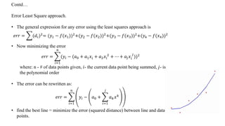
9. Contd…
• Least square regression.
 With linear regression a linear equation, is chosen that fits the data points such that the sum of
the squared error between the data points and the line is minimized
The squared distance is computed with respect to the y – axis.
 Given a set of data points
𝑥 𝑘, 𝑦 𝑘 , 𝑘 = 1, … , 𝑁
The mean squared error (mse) is defined as
𝑚𝑠𝑒 =
1
𝑁
𝐾=1
𝑁
[𝑦 𝑘 − 𝑦1 𝑘]2
=
1
𝑁
𝐾=1
𝑁
[𝑦 𝑘 − (𝑚𝑥 𝑘+𝑏)]2
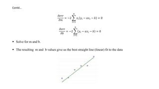
 The minimum mse is obtained for particular values of m and b. Using calculus we compute the
derivative of the mse with respect to both m and b.
1. derivative describes the slope
2. slope = zero is a minimum ==> take the derivative of the

10. Contd…
𝜕𝑒𝑟𝑟
𝜕𝑚
= −2
𝑖=1
𝑛
𝑥𝑖 𝑦𝑖 − 𝑎𝑥𝑖 − 𝑏 = 0
𝜕𝑒𝑟𝑟
𝜕𝑏
= −2
𝑖=1
𝑛
𝑦𝑖 − 𝑎𝑥𝑖 − 𝑏 = 0
 Solve for m and b.
 The resulting m and b values give us the best straight line (linear) fit to the data

11. For higher order polynomials.
• Polynomial curve fitting
• Consider the general form for a polynomial of order 𝑗
𝑓 𝑥 = 𝑎0 + 𝑎1 𝑥 + 𝑎2 𝑥2 + ⋯ + 𝑎𝑗 𝑥 𝑗 = 𝑎0 +
𝑖=1
𝑗
𝑎 𝑘 𝑥 𝑘
• The curve that gives minimum error between data and the fit 𝑓(𝑥) is best.
• Quantify the error for these two second order curves.
• Add up the length of all the red and blue vertical lines.
• Pick curve with minimum total error

12. Contd…
Error Least Square approach.
• The general expression for any error using the least squares approach is
𝑒𝑟𝑟 = (𝑑𝑖)2= (𝑦1 − 𝑓(𝑥1))2+(𝑦2 − 𝑓(𝑥2))2+(𝑦3 − 𝑓(𝑥3))2+(𝑦4 − 𝑓(𝑥4))2
• Now minimizing the error
𝑒𝑟𝑟 =
𝑖=1
𝑛
(𝑦𝑖 − (𝑎0 + 𝑎1 𝑥𝑖 + 𝑎2 𝑥𝑖
2
+ ⋯ + 𝑎𝑗 𝑥𝑖
𝑗
))2
where: n - # of data points given, 𝑖- the current data point being summed, 𝑗- is
the polynomial order
• The error can be rewritten as:
𝑒𝑟𝑟 =
𝑖=1
𝑛
𝑦𝑖 − 𝑎0 +
𝑖=1
𝑗
𝑎 𝑘 𝑥 𝑘
• find the best line = minimize the error (squared distance) between line and data
points.

13. • Overfit
• over-doing the requirement for the fit to ‘match’ the data trend (order too high).
• Picking an order too high will overfit the data.
• Underfit
• If the order is too low to capture obvious trends in the data

14. References:
1. essie.ufl.edu/~kgurl/Classes/Lect3421/Fall_01/NM5_curve_f01
2. collum.chem.cornell.edu/documents/Intro_Curve_Fitting
3. eas.uccs.edu/~mwickert/ece1010/lecture_notes/1010n6a

15. Thank you