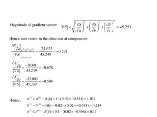
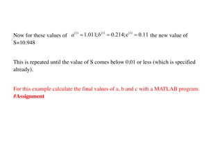
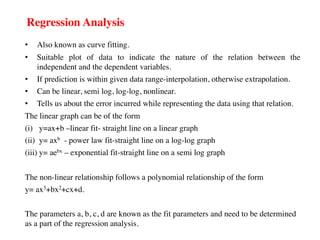
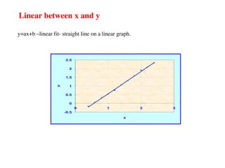
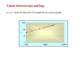
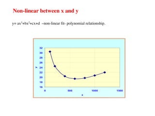
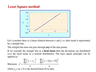
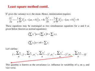
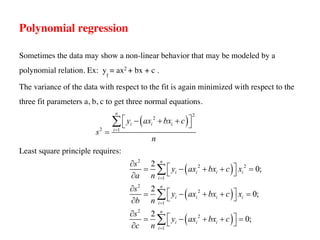
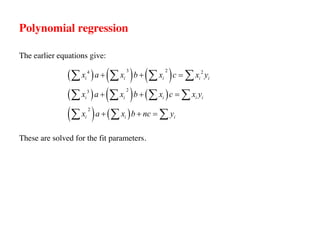
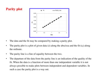
The document discusses regression analysis in thermofluids, covering techniques such as linear, polynomial, and non-linear regression. It explains the least squares method for adjusting fit parameters based on minimizing variance, as well as the calculation of correlation coefficients and standard error to assess fit quality. Additionally, it touches on the concept of parity plots and the general non-linear fitting process, emphasizing the importance of minimizing residuals and determining fit parameters through gradient descent.


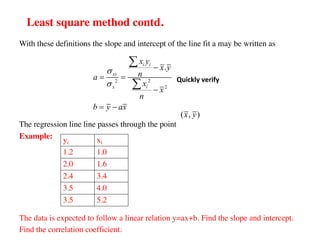
![Standard error
Let’s say the computed value of y is
And suppose there are “n” number of data. Then considering a linear fit we have 2
parameters “a” and “b”.
Hence, DOF = n-p = n-2 [Two parameters a and b are calculated using the same data.]
Hence, standard error is given by:
f
y ax b
= +
[ ]
1/2
2
1
1/2
2
i
1
2
(ax b)
2
n
i f
i
n
i
i
y y
e
n
y
e
n
=
=
ì ü
é ù
-
ï ï
ë û
ï ï
= í ý
-
ï ï
ï ï
î þ
ì ü
- +
ï ï
ï ï
= í ý
-
ï ï
ï ï
î þ
å
å](https://image.slidesharecdn.com/3-regressionanalysis-221023123533-0f02a9d9/85/Regression-Analysis-pdf-10-320.jpg)
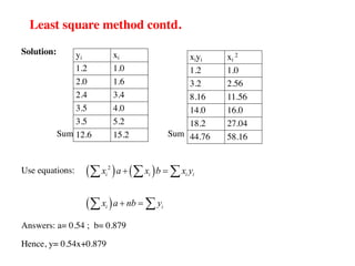
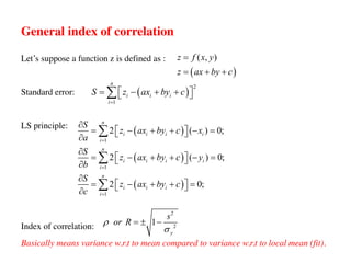
![Goodness of fit and the index of correlation
In the case of a non-linear fit we define a quantity
known as the index of correlation to determine the
goodness of the fit.
[ ]
2
2
2
2
1 1
f
y
y y
s
y y
r
s
é ù
-
ë û
= ± - = ± -
-
å
å
• If the index of correlation is close to ±1, the fit to be considered good.
• The index of correlation is identical to the correlation coefficient for a linear fit.
• The index of correlation compares the scatter of the data with respect to its own
mean as compared to the scatter of the data with respect to the regression curve](https://image.slidesharecdn.com/3-regressionanalysis-221023123533-0f02a9d9/85/Regression-Analysis-pdf-15-320.jpg)
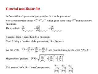
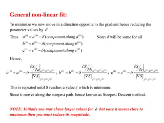
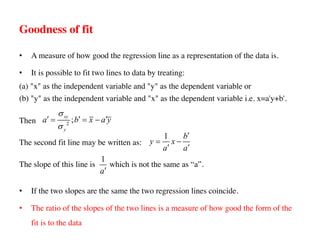
![General non-linear fit:
What if the fit equation is a non-linear relation that is neither a polynomial nor can be
reducible to the linear form?
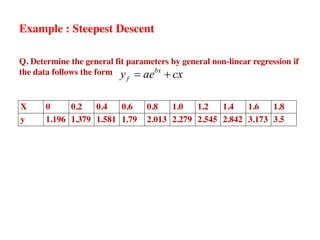
Example:
Here, parameter estimation requires the use of a search method to determine the best
parameter set that minimizes the sum of the squares of the residual. i.e. to find (a,
b,….p) such that S is minimized for yf = f (x : a, b, c….p ) – [general non linear
function with p parameters].
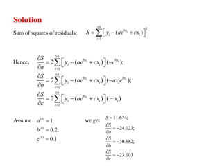
Where sum of the squares of the residual given by
Hence, choose the parameters such that
In general it is not possible to set the partial derivatives with respect to the parameters
to zero to obtain the normal equations and thus obtain the fit parameters.
2
b( ln )
(1) (2)
bx x c x d
y ae cx d or y ae + +
= + + =
2
1
(min)
N
i f
i
S y y
=
é ù
= -
ë û
å
.... 0
S S S S
a b c p
¶ ¶ ¶ 
= = = =
¶ ¶ ¶ ¶](https://image.slidesharecdn.com/3-regressionanalysis-221023123533-0f02a9d9/85/Regression-Analysis-pdf-18-320.jpg)