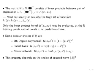
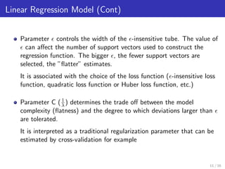
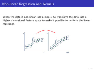
Support Vector Machines can be used for regression by finding the tube that best fits the data while minimizing complexity. This is done by minimizing errors outside an epsilon-insensitive tube while allowing errors within epsilon. Non-linear regression is handled by mapping data into a higher dimensional feature space and using kernels to calculate inner products without explicitly performing the mapping. Kernels allow support vector regression to find a linear function in this feature space, resulting in a non-linear function in the original space.

1. Support Vector Machines for Regression
July 15, 2015
1 / 16

2. Overview
1 Linear Regression
2 Non-linear Regression and Kernels
2 / 16

3. Linear Regression Model
The linear regression model
f(x) = xT
β + β0
To estimate β, we consider minimization of
H(β, β0) =
N
i=1
V (yi − f(xi)) +
λ
2
β 2
with a loss function V and a regularization λ
2 β 2
• How to apply SVM to solve the linear regression problem?
3 / 16

4. Linear Regression Model (Cont)
The basic idea:
Given training data set (x1, y1), ..., (xN , yN )
Target: find a function f(x) that has at most deviation from targets
yi for all the training data and at the same time is as less complex
(flat) as possible.
In other words we do not care about errors as long as they are less
than but will not accept any deviation larger than this.
4 / 16

5. Linear Regression Model (Cont)
• We want to find one ” -tube” that can contains all the samples.
• Intuitively, a tube, with a small width, seems to over-fit with the training
data.
We should find f(x) that its -tube’s width is as big as possible (more
generalization capability, less prediction error in future).
• With a defined , a bigger tube
corresponds to a smaller β
(flatter function).
• Optimization problem:
minimize
1
2
β 2
s.t
yi − f(xi) ≤
f(xi) − yi ≤
5 / 16

6. Linear Regression Model (Cont)
With a defined , this problem is not always feasible, so we also want to
allow some errors.
Use slack variables ξi, ξ∗
i , the
new optimization problem:
minimize
1
2
β 2
+ C
N
i=1
(ξi + ξ∗
i )
s.t



yi − f(xi) ≤ + ξ∗
i
f(xi) − yi ≤ + ξi
ξi, ξ∗
i ≥ 0
6 / 16

7. Linear Regression Model (Cont)
Let λ = 1
C
Use an ” -insensitive” error measure,
ignoring errors of size less than
V (r) =
0 if |r| <
|r| − , otherwise.
We have the minimization of
H(β, β0) =
N
i=1
V (yi − f(xi)) +
λ
2
β 2
7 / 16

8. Linear Regression Model (Cont)
The Lagrange (primal) function:
LP =
1
2
β 2
+ C
N
i=1
(ξ∗
i + ξi) −
N
i=1
α∗
i ( + ξ∗
i − yi + xT
i β + β0)
−
N
i=1
αi(ε + ξi + yi − xT
i β − β0) −
N
i=1
(η∗
i ξ∗
i + ηiξi)
which we minimize w.r.t β, β0, ξi, ξ∗
i . Setting the respective derivatives to
0, we get
0 =
N
i=1
(α∗
i − αi)
β =
N
i=1
(α∗
i − αi)xi
α
(∗)
i = C − η
(∗)
i , ∀i
8 / 16

9. Linear Regression Model (Cont)
Substitute to the primal function, we obtain the dual optimization problem:
max
αi,α∗
i
−
N
i=1
(α∗
i +αi)+
N
i=1
yi(α∗
i −αi)−
1
2
N
i,i =1
(α∗
i −αi)(α∗
i −αi ) xi, xi
s.t



0 ≤ αi, α∗
i ≤ C(= 1/λ)
N
i=1(α∗
i − αi) = 0
αiα∗
i = 0
The solution function has the form
ˆβ =
N
i=1
(ˆα∗
i − ˆαi)xi
ˆf(x) =
N
i=1
(ˆα∗
i − ˆαi) x, xi + β0
9 / 16

10. Linear Regression Model (Cont)
Follow KKT conditions, we have
ˆα∗
i ( + ξ∗
i − yi + ˆf(xi)) = 0
ˆαi( + ξi + yi − ˆf(xi)) = 0
(C − ˆα∗
i )ˆξ∗
i = 0
(C − ˆαi)ˆξi = 0
→ For all data points inside the -tube, ˆαi = ˆα∗
i = 0. Only data points
outside may have (ˆα∗
i − ˆαi) = 0.
→ Do not need all xi to describe β. The associated data points are called
the support vectors.
10 / 16

11. Linear Regression Model (Cont)
Parameter controls the width of the -insensitive tube. The value of
can affect the number of support vectors used to construct the
regression function. The bigger , the fewer support vectors are
selected, the ”flatter” estimates.
It is associated with the choice of the loss function ( -insensitive loss
function, quadratic loss function or Huber loss function, etc.)
Parameter C (1
λ) determines the trade off between the model
complexity (flatness) and the degree to which deviations larger than
are tolerated.
It is interpreted as a traditional regularization parameter that can be
estimated by cross-validation for example
11 / 16

12. Non-linear Regression and Kernels
When the data is non-linear, use a map ϕ to transform the data into a
higher dimensional feature space to make it possible to perform the linear
regression.
12 / 16

13. Non-linear Regression and Kernels (Cont)
Suppose we consider approximation of the regression function in term of a
set of basis function {hm(x)}, m = 1, 2, ..., M:
f(x) =
M
m=1
βmhm(x) + β0
To estimate β and β0, minimize
H(β, β0) =
N
i=1
V (yi − f(xi)) +
λ
2
β2
m
for some general error measure V (r). The solution has the form
ˆf(x) =
N
i=1
ˆαiK(x, xi)
with K(x, x ) = M
m=1 hm(x)hm(x )
13 / 16

14. Non-linear Regression and Kernels (Cont)
Let work out with V (r) = r2. Let H be the N x M basis matrix with imth
element hm(xi) For simplicity assume β0 = 0. Estimate β by minimize
H(β) = (y − Hβ)T
(y − Hβ) + λ β 2
Setting the first derivative to zero, we have the solution ˆy = Hˆβ with ˆβ
determined by
−2HT
(y − Hˆβ) + 2λˆβ = 0
−HT
(y − Hˆβ) + λˆβ = 0
−HHT
(y − Hˆβ) + λHˆβ = 0 (premultiply by H)
(HHT
+ λI)Hˆβ = HHT
y
Hˆβ = (HHT
+ λI)−1
HHT
y
14 / 16

15. Non-linear Regression and Kernels (Cont)
We have estimate function:
f(x) = h(x)T ˆβ
= h(x)T
HT
(HHT
)−1
Hˆβ
= h(x)T
HT
(HHT
)−1
(HHT
+ λI)−1
HHT
y
= h(x)T
HT
[(HHT
+ λI)(HHT
)]−1
HHT
y
= h(x)T
HT
[(HHT
)(HHT
) + λ(HHT
)I]−1
HHT
y
= h(x)T
HT
[(HHT
)(HHT
+ λI)]−1
HHT
y
= h(x)T
HT
(HHT
+ λI)−1
(HHT
)−1
HHT
y
= h(x)T
HT
(HHT
+ λI)−1
y
= [K(x, x1)K(x, x2)...K(x, xN )]ˆα
=
N
i=1
ˆαiK(x, xi)
where ˆα = (HHT
+ λI)−1y. 15 / 16

16. • The matrix N x N HHT
consists of inner products between pair of
observation i, i . {HHT
}i,i = K(xi, xi )
→ Need not specify or evaluate the large set of functions
h1(x), h2(x), ..., hM (x).
Only the inner product kernel K(xi, xi ) need be evaluated, at the N
training points and at points x for predictions there.
• Some popular choices of K are
dth-Degree polynomial: K(x, x ) = (1 + x, x )d
Radial basis: K(x, x ) = exp(−γ x − x 2)
Neural network: K(x, x ) = tanh(κ1 x, x + κ2)
• This property depends on the choice of squared norm β 2
16 / 16