The document discusses curve fitting and modeling. It begins with a quote about fitting an elephant with four parameters. It then discusses searching for the "holy elephant" by fitting data to different models. The rest of the document discusses various aspects of curve fitting such as determining the fitting function, testing accuracy, improving the model, and dealing with issues like nonlinearity and non-constant variance. It emphasizes using techniques like learning curves and bootstrapping to evaluate fit and avoid overfitting. The overall message is that model fitting requires supporting it with residual analysis and having the right balance of model flexibility and data.

1. The Art of Curve Fitting
Anshumaan Bajpai
10/28/2015
1

2. The Rebuke
2
“With four parameters I
can fit an elephant, and
with five I can make him
wiggle his trunk”
Theoretical Physicist,
Cornell University
Freeman Dyson
“I think it's almost true without
exception if you want to win a Nobel
Prize, you should have a long attention
span, get hold of some deep and
important problem and stay with it for
ten years. That wasn't my style”
Enrico Fermi Richard Dawkins
--- John Von Neumann
“Freeman Dyson is in the
tradition of Lord Kelvin &
Fred Hoyle: physicists who
foolishly barge into biology
& pull rank”
Evolutionary Biologist,
University of Oxford
Italian Physicist,
Columbia University
Manhattan Project
 plotted theoretical graphs of
mesonproton scattering
 Calculations agreed with
Fermi’s measured numbers
--- Dawkins on twitter

3. Search for the holy elephant
3
 Neumann made the comment before 1953 but he never
demonstrated how to fit an elephant and neither did Fermi
 Many tried but failed and it wasn’t until 2010 when a
research group from Germany published:

4. Content
 What exactly are we trying to fit?
 Models at our disposal
 Obtaining the fitting function
 Testing the accuracy of model
 Improving the model
4

5. What exactly are we fitting ?
5

6. What exactly are we fitting ?
6

7. What exactly are we fitting ?
7
 Is this model correct ?
 However, what if the data plotted here
was generated using:
 If you answer NO, then the probability
that you are right is very high
𝑌 = 𝑓(𝑋 𝑛)
 Should I go to higher order polynomials ?
 Yes!!
 If I know that my data collection/generation
has no error, and assuming I know its
functional form (polynomial, log, trigonometric
function), the parameters should be tuned to
get the most accurate fit

8. What exactly are we fitting ?
8
 In most practical conditions, there will be
errors in the measurement
 Instrument least count
 Lack of all the variables in the
model
𝑆 =
1
2
𝑔𝑡2
𝑆 =
1
2
𝑔𝑡2 + 𝑓(𝜂)
𝑌 = 𝑓 𝑋
𝑌 = 𝑓 𝑋 + 𝜖
 f represents the systematic information
that X provides about Y, whereas є is the
random error term

9. 9
What exactly are we fitting ?
𝑌 = 𝑓 𝑋3
, 𝑋2
, 𝑋1
, 𝑋0

10. 10
What exactly are we fitting ?
𝑌 = 𝑓 𝑋3
, 𝑋2
, 𝑋1
, 𝑋0

11. 11
What exactly are we fitting ?
𝑌 = 𝑓 𝑋3
, 𝑋2
, 𝑋1
, 𝑋0
+ 𝜖

12. 12
What exactly are we fitting ?
𝑌 = 𝑓 𝑋3
, 𝑋2
, 𝑋1
, 𝑋0
+ 𝜖

13. What exactly are we fitting ?
13
𝑌 = 𝑓 𝑋3
, 𝑋2
, 𝑋1
, 𝑋0
+ 𝜖
Data availableWe need

14. Why Estimate f ?
14
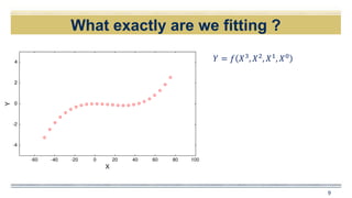
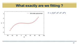
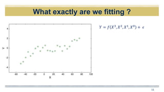
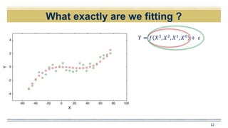
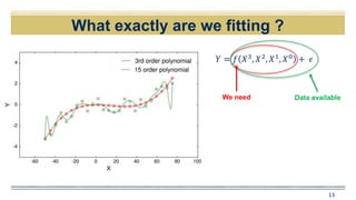
𝑌 = 𝑓 𝑋3
, 𝑋2
, 𝑋1
, 𝑋0
+ 𝜖
Data availableWe need
 Prediction
𝑌′ = 𝑓′ 𝑋
 Inference
 How does Y depend on X ?
 We do need to estimate f but the is
not necessarily to make predictions
on Y
𝐸(𝑌 − 𝑌′)2= 𝐸[𝑓 𝑋 + 𝜖 − 𝑓′(𝑋)]2
= [𝑓 𝑋 − 𝑓′(𝑋)]2+𝑉𝑎𝑟(𝜖)
Reducible Irreducible

15. How do we estimate f ?
15
 Parametric approaches
 Make an assumption about the functional form of f
 Then perform a least square fitting to obtain the parameters
 Easy to estimate the parameters once we assume a certain functional form
 The assumed functional form would usually not match true f
 Non-parametric approaches
 No specific functional form of f is assumed
 Attempt is made to come up with a functional form that fits that data as well as possible without
being too rough
 Is more likely to estimate the true functional form
 Needs lots and lots of data points
𝑓 𝑋 = 𝑎0 + 𝑎1 𝑋 + 𝑎2 𝑋2
+ ⋯ + 𝑎 𝑝 𝑋 𝑝

16. Accuracy vs Interpretability
16An Introduction to statistical learning with Applications in R

17. Is our model accurate ?
17
𝑀𝑒𝑎𝑛 𝑆𝑞𝑢𝑎𝑟𝑒𝑑 𝐸𝑟𝑟𝑜𝑟(𝑀𝑆𝐸) =
1
𝑛
𝑖=1
𝑛
(𝑦𝑖 − 𝑓′
(𝑥𝑖) )2
Training data Testing dataTraining MSE Testing MSE

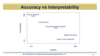
18. Bias-Variance trade off
18
 One basic inference from a U–shaped/Convex dependency ?
𝐸((𝑦0) − 𝑓′(𝑋0))2= 𝑉𝑎𝑟 𝑓′ 𝑋0 + [𝐵𝑖𝑎𝑠(𝑓′ 𝑋0 )]2+𝑉𝑎𝑟(𝜖)
Expected Test MSE
 Flexible methods
 High Variance
 Low bias
 Rigid methods
 High bias
 Low variance

19. Improving the Model
19
 Learning Curves
 Bootstrapping
 Identifying Non linearity in data
 Non constant variance of error terms

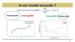
20. Learning Curves
20
Quadratic fit
𝐸((𝑦0) − 𝑓′
(𝑋0))2
= 𝑉𝑎𝑟 𝑓′
𝑋0 + [𝐵𝑖𝑎𝑠(𝑓′
𝑋0 )]2
+𝑉𝑎𝑟(𝜖)
Expected Test MSE High biasHigh var

21. Learning Curves: High Bias
21
Linear fit The model inadequately fits the training data
 Increasing the training set size won’t help
 Need to increase the flexibility of the model

22. Learning Curves: High Variance
22
Gap
 The model overfits fits the training data
 Do not need to increase the model flexibility
 Need to increase the size of training set

23. Bootstrapping
23
𝑌 ≈ 𝛽0 + 𝛽1 𝑋
𝑌′ = 𝛽0
′
+ 𝛽1
′
𝑋
𝛽′
= (𝑥 𝑇
𝑥)−1
𝑥 𝑇
y
Population regression line
 When we assume a linear model:
 We take a sample set from the population:
 Using linear algebra:
𝑅𝑆𝑆 =
𝑖=1
𝑛
(𝑦𝑖 − 𝑦𝑖
′)2
Least square fit
An Introduction to statistical learning with Applications in R

24. Nonlinearity of the data
24An Introduction to statistical learning with Applications in R

25. Non Constant variance of Error terms
25An Introduction to statistical learning with Applications in R

26. Take away message
 Learning Curves are an excellent way to find out if I need more data
or do I need to change our model
 Bootstrapping provides a better estimate of true parameters
 Model fitting should be supported by residual plots, they are always
worth the time
26

27. Thank You
27

28. References:
• Enrico_fermi : http://www.biography.com/people/enrico-fermi-9293405
• Freeman Dyson: https://www.sns.ias.edu/faculty
• Freeman Dyson_happy: http://www.weheartdiving.com/page/3/
• Freeman Dyson _bored: http://jqi.umd.edu/news/phil-schewes-book-published
• Jon Neumann: http://207.44.136.17/celebrity/John_Von_Neumann/
• Art: http://www.pickywallpapers.com/1600x900/miscellaneous/drawings/recursive-hand-drawing-
wallpaper/download/
28