This document discusses nonlinear regression analysis using R. It provides an example of using the nls function to fit nonlinear curves to data. Specifically, it generates random y-data using an exponential decay function of t, plots the data, and performs nonlinear regression to estimate the parameters of the underlying exponential decay model. It also discusses fitting a Gompertz growth curve model to height data using nls. The output is analyzed to test if parameter estimates are statistically significant. Finally, it briefly introduces self-starting nonlinear regression models in R that do not require initial parameter values.

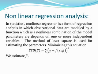
1. Non linear regression analysis:
In statistics , nonlinear regression is a form of regression
analysis in which observational data are modeled by a
function which is a nonlinear combination of the model
parameters are depends on one or more independent
variables . The method of least square is used for
estimating the parameters. Minimizing this equation
푆푆퐷 훽 = Σ 푦 − 푓 푥; 훽
2
We estimate 훽.

2. R code for nonlinear curve fitting
To perform the nonlinear regression analysis in R then
we use nls function.
Example:
t<-seq (0,10,0.1)
y<-rnorm(101,5* exp (-t/5),0.2)
plot(t, y, type="p", pch =16,col="red")

3. Plot :
From the diagram we see that the function is not linear.

4. Now we perform the nonlinear analysis
nls(y~A*exp (-alpha*t),start=c(A=2,alpha=0.05))
summary(nls(y~A*exp(alpha*t),start=c(A=2,alpha=0.05)))
#Using summary we can test the hypothesis whether the
parameters are zero or not.
Outcome:
A alpha
5.0664 0.2025
residual sum-of-squares: 4.436
Number of iterations to convergence: 5

5. Estimate Std. Error t value Pr(>|t|)
A 5.066399 0.062600 80.93 <2e-16 ***
alpha 0.202503 0.004034 50.20 <2e-16 ***
Significance codes: 0 ‘***’ 0.001 ‘**’ 0.01 ‘*’ 0.05 ‘.’ 0.1 ‘ ’ 1
Residual standard error: 0.2117 on 99 degrees of freedom
From the result we see that the p value too small(<0.05)
. so we reject the null hypothesis.

6. Gompertz function….
Gompertz curve or Gompertz function is a type of
mathematical model for a time series. In the Gompartz
curve growth is slowest at the start and end of a time
period. The Gompertz curve has a sigmoidal shape. The
equation is
푦 = 푎푒−푏푒−푔푥

7. Gompertz curve:

8. Fitting Gompertz Curve:
Finding the starting value:
library(ISwR)
juul
attach(subset(juul2,age<20 & age>5 & sex==1))
data.1<-subset(juul2,age<20 & age>5 & sex==1)
attach(data.1)
Now the Gompertz model is a푒−푏푒−푔푥
,the curve has a sigmoidal
shape , approaching a constant level a as x increases and zero for
large negative x. To obtain b and g parameter determined the
location and sharpness. To obtain starting values for a non-linear
fit one approach is to notice that the relation between y and x is
something like log-log linear
log(log(α)-log(y))=log(b)-gx

9. From the figure (juul2), we get the maximum value of height i.e. a=200. With
this guess
we can make a plot that should so an approximate linear relationship.
plot(log(log(200)-log(height))~age, col="blue", pch=16)
fit<-lm(log(log(200)-log(height))~age)
fit
From this we get the value of
log(b)=0.42 and age=-0.1553
Now we fit a nonlinear regression analysis
nls(height~ α * exp (b * exp (-g*age)),start=c(α =200,b= exp (0.4293),g =0.1553))
plot( age, height)
fit<-nls( height~ α*exp(- b *exp(- g *age)),start=c(a=200, b=exp(0.4293),g =0.1553))
Summary(fit)
fit.frame<-seq ( 5,20,0.001)
lines(fit.frame, predict(fit, newdata =data.frame(age=fit.frame)),lwd=2)

11. Outcomes:
After fitting the nls function we get the values of
a b g
242.80628 1.17598 0.07903
then we test the hypothesis that the parameters are zero or not.
Parameters:
Estimate Std. Error t value P(>|t|)
a 2.428e+02 1.157e+01 20.978 <2e-16 ***
b 1.176e+00 1.892e-02 62.149 <2e-16 ***
g 7.903e-02 8.569e-03 9.222 <2e-16 ***
---
Signif. codes: 0 ‘***’ 0.001 ‘**’ 0.01 ‘*’ 0.05 ‘.’ 0.1 ‘ ’ 1
From the result we see that the p values of parameters are too
small(<0.05). so we reject our null hypothesis at 5% level of
significant.

12. Plot the function with respect the sequence.

13. Self starting models:
Doesn't need to input initial values.
This type of functions are starting with SS in R
Ssgompertz.
library(ISwR)
age.height<-subset(juul2,age<20 & age>5 & sex==1)
attach(age.height)
nls(height~ SSgompertz(age,α,b, g ))
α b g
242.807 1.176 0.924
residual sum-of-squares: 23151

14. Draw back of self starting method:
One minor drawback of self starting models is that we can
not just transform them if you want to see if the model fits
better on, e.g. a log-transformation
nls(log(height)~log(SSgompertz(age,α,b,g)))
So we can not use any transformation in self starting model.

15. Thank you……