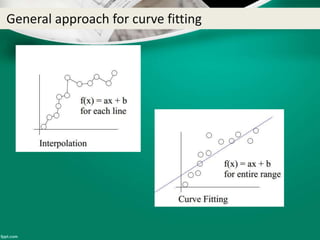
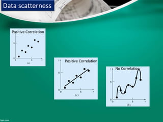
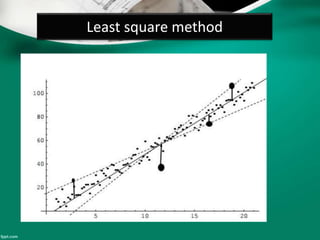
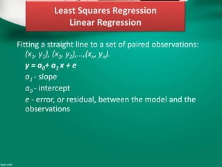
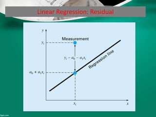
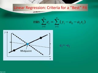
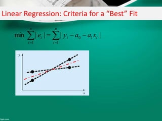
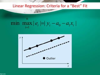
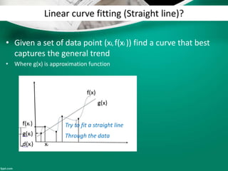
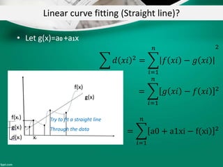
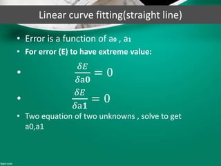
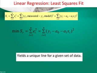
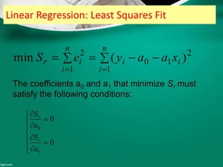
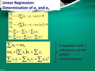
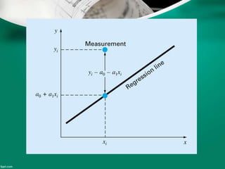
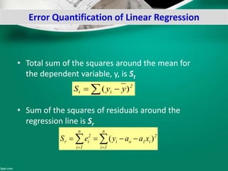
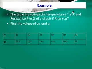
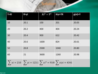
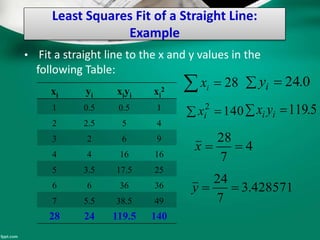
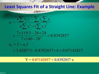
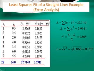
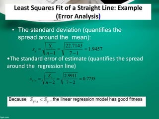
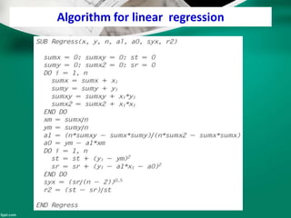
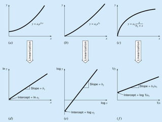
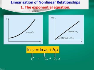
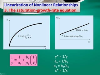
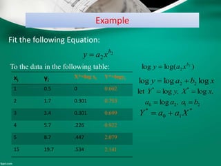
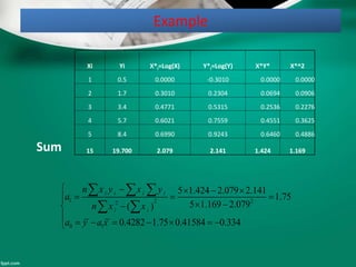
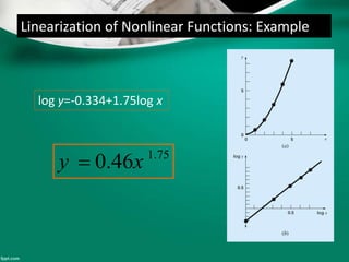
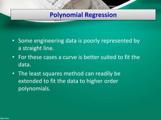
Curve fitting is the process of finding the best fit mathematical function for a series of data points. It involves constructing curves or equations that model the relationship between dependent and independent variables. The least squares method is commonly used, which finds the curve that minimizes the sum of the squares of the distances between the data points and the curve. This provides a single curve that best represents the overall trend of the data. Examples of linear and nonlinear curve fitting are provided, along with the process of linearizing nonlinear relationships to apply linear regression techniques.

1. Curve fitting (Theory & problems)
Session: 2013-14 (Group no: 05)
CEE-149 Credit 02
Curve fitting (Theory & problems)
Numerical Analysis

2. Definition
• Curve fitting: is the process of constructing a curve,
or mathematical function, that has the best fit to a
series of data points, possibly subject to
constraints.
• It is a statistical technique use to drive coefficient
values for equations that express the value of
one(dependent) variable as a function of another
(independent variable)

3. What is curve fitting
Curve fitting is the process of constructing a curve,
or mathematical functions, which possess closest
proximity to the series of data. By the curve fitting
we can mathematically construct the functional
relationship between the observed fact and
parameter values, etc. It is highly effective in
mathematical modelling some natural processes.

4. Interpolation & Curve fitting
• In many application areas, one is faced with the test
of describing data, often measured, with an analytic
function. There are two approaches to this problem:-
• 1. In Interpolation, the data is assumed to be correct
and what is desired is some way to descibe what
happens between the data points.
• 2. The other approach is called curve fitting or
regression, one looks for some smooth curve that
``best fits'' the data, but does not necessarily pass
through any data points.

5. Curve fitting
• There are two general approaches for curve fitting:
• Least squares regression:
Data exhibit a significant degree of scatter. The
strategy is to derive a single curve that represents the
general trend of the data.
Interpolation:
Data is very precise. The strategy is to pass a curve or a
series of curve through each of the points.

6. General approach for curve fitting

7. Engineering applications of curve fitting technique
• 1.Trend Analysis:- Predicating values of dependent
variable ,may include extrapolation beyond data
points or interpolation between data points.

8. Some important relevant parameters
In engineering, two types of applications are encountered:
– Trend analysis. Predicting values of dependent
variable, may include extrapolation beyond data
points or interpolation between data points.
– Hypothesis testing. Comparing existing mathematical
model with measured data.

9. Data scatterness
Positive Correlation
Positive Correlation
No Correlation

10. Mathematical Background
• Arithmetic mean. The sum of the individual data
points (yi) divided by the number of points (n).
Standard deviation. The most common measure of a
spread for a sample.
ni
n
y
y i
,,1, 

 

 2
)(,
1
yyS
n
S
S it
t
y

11. Mathematical Background (cont’d)
• Variance. Representation of spread by the square of
the standard deviation.
• Coefficient of variation. Has the utility to quantify
the spread of data.
1
)( 2
2




n
yy
S i
y
 
1
/
22
2



 
n
nyy
S ii
y
%100..
y
S
vc
y


12. Least square method
• The Method of Least Squares is a procedure to determine
the best fit line to data; the
proof uses simple calculus and linear algebra. The basic
problem is to find the best fit
straight line y = ax + b given that, for n ∈ {1, . . . , N}, the
pairs (xn, yn) are observed.
The method easily generalizes to finding the best fit of the
form
y = a1f1(x) + · · · + cKfK(x);
it is not necessary for the functions fk to be linearly in x –
all that is needed is that y is to
be a linear combination of these functions.

13. Least square method

14. Least Squares Regression
Linear Regression
Fitting a straight line to a set of paired observations:
(x1, y1), (x2, y2),…,(xn, yn).
y = a0+ a1 x + e
a1 - slope
a0 - intercept
e - error, or residual, between the model and the
observations

15. Linear Regression: Residual

16. Linear Regression: Criteria for a “Best” Fit
 

n
i
ii
n
i
i xaaye
1
10
1
)(min
e1= -e2

17. Linear Regression: Criteria for a “Best” Fit
 

n
i
ii
n
i
i xaaye
1
10
1
||||min

18. Linear Regression: Criteria for a “Best” Fit
||||maxmin 10
n
1i
iii xaaye 


19. Linear curve fitting (Straight line)?
• Given a set of data point (xi, f(xi )) find a curve that best
captures the general trend
• Where g(x) is approximation function
Try to fit a straight line
Through the data

20. Linear curve fitting (Straight line)?
• Let g(x)=a0 +a1x
𝑑 𝑥𝑖 2 =
𝑖=1
𝑛
𝑓 𝑥𝑖 − 𝑔 𝑥𝑖
2
=
𝑖=1
𝑛
𝑔 𝑥𝑖 − 𝑓 𝑥𝑖 2
=
𝑖=1
𝑛
a0 + a1xi − f(xi 2
Try to fit a straight line
Through the data

21. Linear curve fitting(straight line)
• Error is a function of a0 , a1
• For error (E) to have extreme value:
•
𝛿𝐸
𝛿a𝟎
= 0
•
𝛿𝐸
𝛿a𝟏
= 0
• Two equation of two unknowns , solve to get
a0,a1

22. Linear Regression: Least Squares Fit
   

n
i
n
i
iiii
n
i
ir xaayyyeS
1 1
2
10
2
1
2
)()model,measured,(
 

n
i
ii
n
i
ir xaayeS
1
2
10
1
2
)(min
Yields a unique line for a given set of data.

23. Linear Regression: Least Squares Fit
 

n
i
ii
n
i
ir xaayeS
1
2
10
1
2
)(min
The coefficients a0 and a1 that minimize Sr must
satisfy the following conditions:













0
0
1
0
a
S
a
S
r
r

24. Linear Regression:
Determination of ao and a1
 
 
 










2
10
10
1
1
1
0
0
0)(2
0)(2
iiii
ii
iioi
r
ioi
o
r
xaxaxy
xaay
xxaay
a
S
xaay
a
S
 
 





2
10
10
00
iiii
ii
xaxaxy
yaxna
naa 2 equations with 2
unknowns, can be
solved
simultaneously

25. Linear Regression:
Determination of ao and a1
  
  


 221
ii
iiii
xxn
yxyxn
a
xaya 10 

27. Error Quantification of Linear Regression
• Total sum of the squares around the mean for
the dependent variable, y, is St
• Sum of the squares of residuals around the
regression line is Sr
  2
it yyS )(
2
n
1i
i1oi
n
1i
2
ir xaayeS )( 


28. Example
• The table blew gives the temperatures T in C and
Resistance R in Ω of a circuit if R=a0 + a1T
• Find the values of a0 and a1
T 10 20 30 40 50 60
R 20.1 20.2 20.4 20.6 20.8 21

29. Solution
T=Xi R=yi 𝑿𝒊 𝟐
= 𝑻 𝟐 Xiyi=TR g(xi)=Y
10 20.1 100 201 20.05
20 20.2 400 404 20.24
30 20.4 900 612 20.42
40 20.6 1600 824 20.61
50 20.8 2500 1040 20.80
60 21 3600 1260 20.98
𝑥𝑖 = 210 𝑦𝑖 = 123.1 𝑥𝑖2
= 9100 𝑥𝑖𝑦𝑖 = 4341

30. Solution
• 6a0+210a1=123.1 a0=19.867
• 210a0+9100a1=4341 a1 =0.01857
• g(x)=19.867+0.01857*T

31. Least Squares Fit of a Straight Line:
Example
• Fit a straight line to the x and y values in the
following Table:
28 ix 0.24 iy
1402
 ix 5.119 ii yx
3
7
24
4
7
28
 yx
428571.3
7
24
4
7
28
 yx
xi yi xiyi xi
2
1 0.5 0.5 1
2 2.5 5 4
3 2 6 9
4 4 16 16
5 3.5 17.5 25
6 6 36 36
7 5.5 38.5 49
28 24 119.5 140

32. Least Squares Fit of a Straight Line: Example
07142857.048392857.0428571.3
8392857.0
281407
24285.1197
)(
10
2
221









 
  
xaya
xxn
yxyxn
a
ii
iiii
Y = 0.07142857 + 0.8392857 x

33. Least Squares Fit of a Straight Line: Example
(Error Analysis)
9911.2
2
  ir eS
868.02



t
rt
S
SS
r
  7143.22
2
  yyS it
932.0868.02
 rr

34. Least Squares Fit of a Straight Line: Example
(Error Analysis)
• The standard deviation (quantifies the
spread around the mean):
9457.1
17
7143.22
1





n
S
s t
y
•The standard error of estimate (quantifies the spread
around the regression line)
7735.0
27
9911.2
2
/ 




n
S
s r
xy

35. Algorithm for linear regression

36. Linearization of Nonlinear Relationships
• The relationship between the dependent and
independent variables is linear.
• However, a few types of nonlinear functions can
be transformed into linear regression problems.
 The exponential equation.
 The power equation.
 The saturation-growth-rate equation.

38. Linearization of Nonlinear Relationships
1. The exponential equation.
xbay 11lnln 
y* = ao + a1 x

39. Linearization of Nonlinear Relationships
2. The power equation
xbay logloglog 22 
y* = ao + a1 x*

40. Linearization of Nonlinear Relationships
3. The saturation-growth-rate equation







xa
b
ay
111
3
3
3
y* = 1/y
ao = 1/a3
a1 = b3/a3
x* = 1/x

41. Example
Fit the following Equation:
2
2
b
xay 
To the data in the following table:
xi yi
X*=log xi Y*=logyi
1 0.5 0 0.602
2 1.7 0.301 0.753
3 3.4 0.301 0.699
4 5.7 .226 0.922
5 8.7 .447 2.079
15 19.7 .534 2.141
)log(log 2
2
b
xay 
2120
**
log
logloglet
b, aaa
x,y, XY


xbay logloglog 22 
*
10
*
XaaY 

42. Example
Xi Yi X*i=Log(X) Y*i=Log(Y) X*Y* X*^2
1 0.5 0.0000 -0.3010 0.0000 0.0000
2 1.7 0.3010 0.2304 0.0694 0.0906
3 3.4 0.4771 0.5315 0.2536 0.2276
4 5.7 0.6021 0.7559 0.4551 0.3625
5 8.4 0.6990 0.9243 0.6460 0.4886
Sum 15 19.700 2.079 2.141 1.424 1.169
1 2 22
0 1
5 1.424 2.079 2.141
1.75
5 1.169 2.079( )
0.4282 1.75 0.41584 0.334
i i i i
i i
n x y x y
a
n x x
a y a x
    
  
 

      
  
 

43. Linearization of Nonlinear Functions: Example
log y=-0.334+1.75log x
1.75
0.46y x

44. Polynomial Regression
• Some engineering data is poorly represented by
a straight line.
• For these cases a curve is better suited to fit the
data.
• The least squares method can readily be
extended to fit the data to higher order
polynomials.

45. Polynomial Regression (cont’d)
A parabola is preferable

46. Polynomial Regression (cont’d)
• A 2nd order polynomial (quadratic) is defined by:
• The residuals between the model and the data:
• The sum of squares of the residual:
exaxaay o  2
21
2
21 iioii xaxaaye 
  
22
21
2
iioiir xaxaayeS

47. Polynomial Regression (cont’d)
0xxaxaay2
a
S
0xxaxaay2
a
S
0xaxaay2
a
S
2
i
2
i2i1oi
2
r
i
2
i2i1oi
1
r
2
i2i1oi
o
r












)(
)(
)(
 
 




4
i2
3
i1
2
ioi
2
i
3
i2
2
i1ioii
2
i2i1oi
xaxaxayx
xaxaxayx
xaxaany 3 linear equations with
3 unknowns (ao,a1,a2),
can be solved

48. Polynomial Regression (cont’d)
• A system of 3x3 equations needs to be solved to determine
the coefficients of the polynomial.
• The standard error & the coefficient of determination
3
/


n
S
s r
xy
t
rt
S
SS
r

2





































ii
ii
i
iii
iii
ii
yx
yx
y
a
a
a
xxx
xxx
xxn
2
2
1
0
432
32
2

49. Polynomial Regression (cont’d)
General:
The mth-order polynomial:
• A system of (m+1)x(m+1) linear equations must be solved for
determining the coefficients of the mth-order polynomial.
• The standard error:
• The coefficient of determination:
exaxaxaay m
mo  .....2
21
 1
/


mn
S
s r
xy
t
rt
S
SS
r

2

50. Polynomial Regression- Example
Fit a second order polynomial to data:
2253
 ix
9794
 ix
xi yi xi
2 xi
3 xi
4 xiyi xi
2yi
0 2.1 0 0 0 0 0
1 7.7 1 1 1 7.7 7.7
2 13.6 4 8 16 27.2 54.4
3 27.2 9 27 81 81.6 244.8
4 40.9 16 64 256 163.6 654.4
5 61.1 25 125 625 305.5 1527.5
15 152.6 55 225 979 585.6 2489
6.585 ii yx
15 ix
6.152 iy
552
 ix
433.25
6
6.152
,5.2
6
15
 yx 8.2488
2
 ii yx

51. 2nd order polynomial Example
2
21 xaxaay o 
xi fi 𝑥𝑖2
𝒙𝒊 𝟑 𝒙𝒊 𝟒 fixi 𝒇𝒊𝒙𝒊 𝟐 g (x)
1 4 1 1 1 4 4 4.505
2 11 4 8 6 22 44 10.15
4 19 16 64 256 76 304 19.43
6 26 36 216 1296 156 936 26.03
8 30 64 512 4096 240 1920 29.95
𝑥 = 21
𝑓𝑖 =
90
𝑥𝑖2
=
121
𝑥𝑖3
= 801
𝑥𝑖4
= 5665
𝑓𝑖𝑥𝑖 =
498
𝑓𝑖𝑥𝑖2
= 3208

52. 2nd order polynomial Example
5a0 +21a1+121a2=90
21a0+121a1+801a2=498
121a0+801a1+5665a2=3208
a0=-1.81 ,a1=6.65 ,a2=-0.335
So the required equation is
g (x)=-1.81+6.65X-0.335𝑥2

53. Exponential function
x 1 2 3 4 5
y 1.5 4.5 6 8.5 11
Solution
y=a𝑒 𝑏𝑥
lny=lna𝑒 𝑏𝑥
=lna+bx
Y=a0+a1X
Where Y=lny=fi, a0=a ,a1=b , X=x

54. X= xi yi Y=lny 𝒙𝒊 𝟐 xiyi g (x)
1 1.5 0.405 1 0.405 2.06
2 4.5 1.504 4 3.008 3.27
3 6 1.791 9 5.373 5.186
4 8.5 2.14 16 8.56 8.22
5 11 2.39 25 11.95 13.03
𝑥𝑖 = 15
𝑓𝑖 =
8.23
𝑥𝑖2 = 55
𝑓𝑖𝑥𝑖 = 29.296
Solution

55. Solution
• 5a0 +15a1 =8.23 ; a0= 0.2642
• 15a0 + 55a1 = 29.296 ;a1=0.4606
• a= 𝑒0.2642=1.30234, b=0.4606
• Require equation g (x)=1.30238𝑒0.4606

56. Example
• Power function:
• y=a𝑥 𝑏
• lny = lna + blnx
• Y=a0 +a1X
• Where, Y=lny, a0=lna; X=lnx; a1=b
x 2 2.5 3 3.5 4
y 7 8.5 11 12.75 15
Solution:

57. Solution
x y lnx=X lny=Y 𝑿 𝟐 XY g (x)
2 7 0.6931 1.946 0.480 1.3487 6.868
2.5 8.5 0.9163 2.140 0.8396 1.9608 8.813
3 11 1.098 2.397 1.2056 2.6319 10.806
3.5 12.75 1.252 2.545 1.5675 3.1863 12.838
4 15 1.386 2.708 1.9209 3.7532 14.904
𝑋𝑖 =
5.3454
𝑓𝑖 =
11.736
𝑋𝑖2 =
6.0136
𝑓𝑖𝑋𝑖 =
12.8809

58. Solution
• 5a0+5.3454a1=11.736
• 5.3454a0+6.0136a1=12.8809
• a0=1.1521 ; a1=1.1178
• a= 𝑒 𝑎0
• =𝑒1.1521
=3.1648
b=a1=1.1178
Required equation=3.1648𝑥1.1178

59. Polynomial Regression- Example (cont’d)
• The system of simultaneous linear equations:
2
210
86071.135929.247857.2
86071.1,35929.2,47857.2
xxy
aaa

































8.2488
6.585
6.152
97922555
2255515
55156
2
1
0
a
a
a
74657.3
2
  ir eS  39.2513
2
  yyS it

60. Polynomial Regression- Example (cont’d)
xi yi ymodel ei
2 (yi-y`)2
0 2.1 2.4786 0.14332 544.42889
1 7.7 6.6986 1.00286 314.45929
2 13.6 14.64 1.08158 140.01989
3 27.2 26.303 0.80491 3.12229
4 40.9 41.687 0.61951 239.22809
5 61.1 60.793 0.09439 1272.13489
15 152.6 3.74657 2513.39333
•The standard error of estimate:
•The coefficient of determination:
12.1
36
74657.3
/ 

xys
99925.0,99851.0
39.2513
74657.339.2513 22


 rrr

61. Reference
• Introduction Method of Numerical Analysis
(S.S Sastry) Page: 126-175
• Numerical methods for engineers ( Steven c.
Chapra, Raymond p. canale) page: 561-69
• https://en.wikipedia.org/wiki/Curve_fitting
• http://site.iugaza.edu.ps/iismail/files/Ch17-
curve-fitting.ppt
• http://caig.cs.nctu.edu.tw/course/NM07S/slide
s/chap3_1.pdf

62. Reference
• http://www.eas.uccs.edu/wickert/ece1010/lectu
re_notes/1010n6a.PDF
• http://www.chee.uh.edu/sites/chbe.egr.uh.edu/f
iles/files/CHEE3334.pdf
• Lecture Sheet of (Dr. Md. Shahidur Rahman
• Assistant Pro. CEE, SUST)

63. THE END
THANK FOR BEING
WITH US