This document discusses numerical methods for solving initial value problems for ordinary differential equations. It introduces the Taylor series method and Runge-Kutta method for solving initial value problems. Examples are provided to demonstrate solving first and second order differential equations using these two methods and to compare their results. Stability of numerical solutions is also discussed.

1. Initial Value Problems
Ali jan
M. Sc Previous (Semester-II)

2. Outline
Taylor
Series
Runge
Kutta
Method
Stability

3. Introduction
• The general form of the 1st order differential
equation is
• Integrating the above equation we get a constant ‘c’,
to find that value, we must know an initial condition,
that is the value of ‘y’ at ‘x’. Let the initial value is
‘x=a’

4. Continue
• An ordinary differential equation of order ‘n’:
• Can always transform into ‘n’ first order equation:
• The equivalent first-order equations are:
• The solution now requires the knowledge ‘n’ auxiliary conditions. If there
conditions are specified at the same value of ‘x=a’, the problem is said to be an
initial value problem. The auxiliary conditions, called initial conditions:
• For example,

5. Taylor Series
• Taylor series method is use to gain high accuracy . Its basis is the truncated Taylor
series for y about x, it is also a formula for numerical integration:
• The last term determines the order of integration, the “truncation error”, due to
the terms omitted from the series:
• Using the finite difference approximation:
• We obtain the more useful form:

6. Continue
• The Taylor function implements the Taylor series method of
integration of order four. It can handle any number of first-order
differential equation:
• The user is required to supply the function “derivative” that
returns the 4 x n matrix:

7. Graphical Representation

8. Working of Taylor Series

9. Continue
• Example 7.1
h=0.1
• The Taylor Series
• Differentiation of the differential equation, yields

10. Continue
at x=0 and y=1
With h=0.1 and substituting the values of derivatives, the above equation becomes

11. Continue
The approximate truncation error:
Therefore
The analytic solution of the differential equation:

12. • Example 7.2
Continue
• From x = 0 to 2 and h=0.25.
• With the notation the equivalent first order equations
and the initial conditions are
• Repeated differentiation of the differential equation yields

13. Continue
Thus the derivative array that has to be computed is

14. Code of Taylor Series
1. from numpy import *
2. def taylor(x, y, n, h):
3. X = [ ]
4. Y = [ ]
5. X.append(x)
6. Y.append(y)
7. for i in range (n) :
8. D = f(x,y)
9. H = 1.0
10. for j in range (4) :
11. H = H * h/(j+1)
12. y = y + D[j] *H
13. x = x + h
14. X.append(x)
15. Y.append(y)
16. print array(X), array(Y)
17. return array (X), array(Y)
18. def f (x,y):
19. D = zeros ((4,2))
20. D [0] = [ y[1], -0.1*y[1]-x ]
21. D [1]=[ D[0,1], 0.01*y[1]+0.1*x-1.0 ]
22. D [2]=[ D[1,1], -0.00*y[1]-0.01*x+0.1 ]
23. D [3]=[ D[2,1], 0.0001*y[1]+0.001*x-0.01 ]
24. return D
25. taylor( 0.0, array ([0.0,1.0]) ,8 , 0.25 )

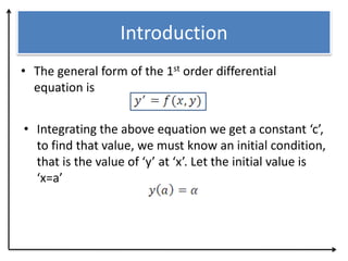
15. The results for Taylor series are:
Continue
x y[0] y[1]
0 0 1
0.25 0.24431315 0.94432131
0.5 0.46713137 0.82829196
0.75 0.65355402 0.65340186
1 0.78904832 0.42110415
1.25 0.85944028 0.13281605
1.5 0.85090579 -0.21008015
1.75 0.74996208 -0.60623633
2 0.54345919 -1.05433763

16. Runge-Kutta Method
• The need for Runge-Kutta Method increased,
because of a drawback of Taylor series.
• Taylor series requires repeated differentiation
of the dependent variables.
• There is extra work of coding each of the
derivatives.
• Runge-Kutta method is used to eliminate the
need for repeated differentiation of the
differential equations.

17. Runge-Kutta Graph

18. RRuunnggee--KKuuttttaaMmeetthhoodd ooff FFoouurrtthh oOrrddeerr
Example no. 7.4
From x = 0 to 2 and h=0.25.
With the notation the equivalent first order equations and the
initial conditions are

19. Code of Runge-Kutta
1. from numpy import *
2. from math import *
3. def run_kutta(x, y, h,n):
4. def run_kut4(x,y,h):
5. k0=h*f(x,y)
6. k1=h*f(x+h/2.0, y+k0/2.0)
7. k2=h*f(x+h/2.0, y+k1/2.0)
8. k3=h*f(x+h, y+k2)
9. return (k0 + 2.0*k1 + 2.0*k2 + k3)/6.0
10. X=[]
11. Y=[]
12. X.append(x)
13. Y.append(y)
14. while x<n:
15. y=y+run_kut4(x,y,h)
16. x=x+h
17. X.append(x)
18. Y.append(y)
19. print array(X), array(Y)
20. return array(X), array(y)
21. def f(x,y):
22. f=zeros((2))
23. f[0]=y[1]
24. f[1]=-0.1*y[1]-x
25. return f
26. run_kutta (0.0,array([0.0,1.0]),0.25,2.0)

20. Continue
The results for Runge-Kutta:
x y[0] y[1]
0 0 1
0.25 0.24431315 0.94432131
0.5 0.46713137 0.82829196
0.75 0.65355402 0.65340186
1 0.78904832 0.42110415
1.25 0.85944028 0.13281605
1.5 0.85090579 -0.21008015
1.75 0.74996208 -0.60623633
2 0.54345919 -1.05433763

21. Stability
• A numerical integration is said to be stable if
the effects of local errors do not accumulate
catastrophically.
• If method is unstable, the global error will
increase exponentially, eventually causing
numerical overflow.
• Stability has nothing to do with accuracy, in
fact, an inaccurate method can be very stable.

22. Continue
• Consider the linear problem
• Where ‘λ’ is a positive constant. The numerical solution:
• Substituting we get
• If “І1- λ І>1”, the method is clearly unstable since ‘y’ increases
in every integration step. Thus it is stable only if “І1- λ І<1”.

23. Miscellaneous
Example 7.6
A Spacecraft is launched at an altitude ‘H=772’ km above sea level with the speed
‘v0=6700 m/s’ in the direction shown. The differential equations describing the
motion of the spacecraft are
‘r’ and ‘θ’ are polar coordinates of spacecraft.
G= 6.672 × 10−11 m3kg−1s−2 = universal gravitational constant
Me= 5.9742 × 1024 kg = mass of the earth
Re = 6378.14 km = radius of the earth at sea level

24. Continue
So, we have
Let
then

25. Continue

26. Code
1. from numpy import *
2. from math import *
3. def integrate(x, y, h,n):
4. def run_kut4(x,y,h):
5. k0=h*f(x,y)
6. k1=h*f(x+h*0.5, y+k0*0.5)
7. k2=h*f(x+h*0.5, y+k1*0.5)
8. k3=h*f(x+h, y+k2)
9. return (k0 + 2.0*k1 + 2.0*k2 + k3)/6.0
10. X=[]
11. Y=[]
12. X.append(x)
13. Y.append(y)
14. while x<n:
15. y=y+run_kut4(x,y,h)
16. x=x+2*h
17. X.append(x)
18. Y.append(y)
19. print array(X), array(Y)
20. return array(X), array(y)
21.f=zeros((4))
22. f[0]=y[1]
23. f[1]=(y[0]*(y[3]**2) - 3.9860e14)/(y[0]**2)
24. f[2]=y[3]
25. f[3]=(-2.0*y[1]*y[3])/y[0]
26. return f
27.Integrate (0.0,array([7.15014e6,0,0,0.937045e-3]),50.,1200.)

27. Result
X=t(s) r=y[0](m) r’=y[1](m) θ =y[2](rad) θ’ =y[3](rad)
0 7.15E+06 0.00E+00 0.00E+00 9.37E-04
100 7.14E+06 -3.90E+02 4.69E-02 9.40E-04
200 7.11E+06 -7.83E+02 9.40E-02 9.47E-04
300 7.06E+06 -1.18E+03 1.42E-01 9.61E-04
400 6.99E+06 -1.58E+03 1.90E-01 9.80E-04
500 6.90E+06 -2.00E+03 2.40E-01 1.01E-03
600 6.79E+06 -2.42E+03 2.91E-01 1.04E-03
700 6.66E+06 -2.86E+03 3.44E-01 1.08E-03
800 6.51E+06 -3.32E+03 3.99E-01 1.13E-03
900 6.33E+06 -3.80E+03 4.57E-01 1.20E-03
1000 6.13E+06 -4.32E+03 5.19E-01 1.28E-03
1100 5.90E+06 -4.87E+03 5.85E-01 1.38E-03
1200 5.64E+06 -5.47E+03 6.57E-01 1.51E-03