this book is prepared by mechanical student in University Of Gondar second year Abdrehman Ahmed

1. Bisection method
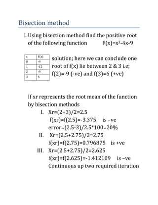
1.Using bisection method find the positive root
of the following function F(x)=x3-4x-9
solution; here we can conclude one
root of f(x) lie between 2 & 3 i.e;
f(2)=-9 (-ve) and f(3)=6 (+ve)
If xr represents the root mean of the function
by bisection methods
I. Xr=(2+3)/2=2.5
f(xr)=f(2.5)=-3.375 is –ve
error=(2.5-3)/2.5*100=20%
II. Xr=(2.5+2.75)/2=2.75
f(xr)=f(2.75)=0.796875 is +ve
III. Xr=(2.5+2.75)/2=2.625
f(xr)=f(2.625)=-1.412109 is –ve
Continuous up two required iteration
x F(x)
0 -9
1 -12
2 -9
3 6

2. Secant method
xi+1=xi-[f(xi)(xi-1-xi)]/[f(xi-1)-f(xi)]
1.Use the secant method to estimate the root of
f(x)=x3-x-1 with initial estimates of 1&2 having
three iteration
Solution;
xi-1=1 and f(2)=5
I. X1=2-[f(2)(1-2)]/[f(1)-f(2)]=2-[5(-1)]/[-1-5] = 1.166667
Now xi-1=2 and xi=1.166667
error= [1.166667-2]/1.166667*100= 71.4286%
II. F(2)=5 and f(1.166667)= -0.5787
X2=1.166667-[-0.5787(2-1.166667)]/[5-(-0.5787)] = 1.25311
Now xi-1 = 1.166667 and xi = 1.25311
III. F(1.166667)=-0.5787 and f(1.25311)= -0.28537
X3 = 1.25311-[-0.28537(1.16667-1.25311)]/[-0.5787-(-0.28537)]
X3= 1.3372 f(1.3372) = 0.0538854

3. Lease square regression method
1.Find the equation of straight line which best fits
n = 7 ,
Ẋ = ∑xi/n
Ý= ∑yi/n ,
a1=[n∑xiyi-∑yi]/[n∑xi2-(∑xi)2
ao = Ý-a1Ẋ
therefore the line which fits the given tabular
points is y= ao+a1x
x 10 12 13 16 17 20 25
y 10 22 24 27 29 33 37
Xi Yi XiYi xi2
10 10 100 100
12 22 264 144
13 24 312 169
16 27 432 256
17 29 493 289
20 33 660 400
25 37 925 625
Sum 113 182 3186 1983

4. Fourier approximation
1.The PH in a reactor varies sinusoidally as the couse
of a day use Fourier approximation
Time(h) 0 2 4 5 7 8.5 12 15 20 22 24
PH 7.3 7 7.1 6.4 7.2 8.9 8.8 8.9 7.9 7.9 7
Where f=1/t and t=24hr , f=1/24= 0.042hr-1 ,n = 11
Wo=2πf=0.261799388
Ao=∑y/n, A1 = 2/n[∑ycos(wot) ,
B1 = 2/n[∑ysin(wot)
The equation will be y= Ao+A1cos(wot)+B1sin(wot)
time(t) PH(y) ycos(wot) ysin(wot)
0 7.3 7.3 0
2 7 6.062177825 3.500000002
4 7.1 3.549999995 6.14878037
5 6.4 1.656441882 6.18192529
7 7.4 -1.915260944 7.147851112
8.5 7.2 -4.383082299 5.712144043
12 8.9 -8.9 -2.14508E-08
15 8.8 -6.222539656 -6.222539693
20 8.9 4.450000031 -7.707626076
22 7.9 6.841600707 -3.94999997
24 7 7 3.37429E-08
Sum 83.9 15.43933754 10.81053509

5. Linear interpolation
The general formula for linear interpolation is
𝑓1( 𝑥)−𝑓(𝑋𝑜)
𝑋−𝑋𝑂
=
f(X1)−f(Xo)
𝑋1−𝑋0
from the above we get the
general formula for linear interpolation
f1(x) = 𝑓(𝑥𝑜) +
𝑓( 𝑥1) − 𝑓( 𝑥𝑜)
𝑥1 − 𝑥𝑜
(𝑥 − 𝑥𝑜)
Example find the value of ln(2) if ln(1)=0 and
ln(4)=1.386294 using linear interpolation
Solution 1st we make a table
Given f(xo)=0, xo=1
f(x1)=1.386294, x1=4
f1(x)=?, x=2
By using linear interpolation formula
f1(x) = 𝑓(𝑥𝑜) +
𝑓( 𝑥1) − 𝑓( 𝑥𝑜)
𝑥1 − 𝑥𝑜
(𝑥 − 𝑥𝑜)
f1(x) = 0 +
1.386294 − 0
4 − 1
(2 − 1)
f1(x) =
1.386294
3
= 0.4621 𝑎𝑛𝑠𝑤𝑒𝑟
x ln(x)
1 0
2 ?
4 1.386294

6. The gauss seidel method
Rule
|a11|>|a12|+|a13|,
|a22|>|a21|+|a23|, and
|a33|>|a31|+|a32|
Iteration 1, y = z =0, xi=?,
x = xi, z = 0 , yi = ?
x = xi, y = yi, zi = ?
Iteration 2,
using yi & zi we get xii = ?
xii & yi we get yii = ?
xii & yii we get zii = ?
continue this to the required iteration
a11 a12 a13
a21 a22 a23
a31 a32 a33
e
f
g

7. The naïve gauss elimination method
Example; given 20x+y+4z=25----------------eq(1)
8x+13y+2z=23--------------eq(2)
4x-11y+21z=14-------------eq(3)
with the value of x=y=z=1
Solution: by multiplying eq(1) by 8/20 and subtract
from eq(2) and also multiply eq(1) by 4/20 and
subtract from eq(3) we get the following set of equations
20x+y+4z=25--------------------eq(1)
12.6y+0.4z=13------------------eq(4)
-11.2y+20.2z=9-------------------eq(5)
by proceeding to eliminate we find a single variable z by multiplying
eq(4) by -11.2/12.6 and subtract from eq(5) we get
20.5556z=20.5556----------------eq(6)
finally we rearrange the equation and written as
20x+y+4z=25 -----------------eq(1)
12.6y+0.4z=13 ----------------eq(4)
20.5556z=20.5556-----eq(6)
now by using back substitution we get the unknowns x,y&z
from eq(6) we get z=1 ,
from eq(4) we get y=1,
from eq(1) we get x=1

8. LU decomposition
© to find the LU decomposition first we find f21=
a21/a11 f31= a31/a11 f32 = a’32/a’22
And the multiplying the first row by f21 and
then subtract this value from second row
Multiplying the first row by f31 and then
subtract this value from third row
Now we find f32 from the matrix we get above
Now multiplying the new matrix second row
by f32 and then subtract this value from the
new matrix row three
Finally we get [U] = [L] =
a11 a12 a13
a21 a22 a23
a31 a32 a33
a11 a12 a13
0 a22 a23
0 0 a33
1 0 0
f21 1 0
f31 f32 1

9. Matrix inverse using LU decomposition
We find the LU decomposition of the given matrix as the
above form and then we find the inverse of the matrix
Procedure one; [L] =
to find the value of d1,d2,d3 by using forward
substitution
d1+0+0=1 we get d1
F21d1+d2+0=0 we get d2
F31d1+F32d2+d3=0 we get d3
the vector can be then used as the right hand side for
the upper triangular matrix
[U] =
let us find the value of x1,x2 and x3 using backward
substitution
0+0+a33x3=d3 from this we get x3
0+a22x2+a23x3=d2 from this we get x2
a11x1+a12x2+a13x3=d1 from this we get x1
d1
d2
d3
1
0
0
d1
d2
d3
x1
x2
x3

10. x1,x2 and x3 are the first column of the inverse matrix
As like as procedure one we get all the columns of the
inverse matrix by only changing
To and using in procedure 2 and 3
respectively
finally the inverse of the matrix we get is
[A]-1 =
1
0
0
0
1
0
0
0
1
X1 X1 X1
X2 X2 X2
X3 X3 X3

11. Trapezoidal rule
Examples;
∫0
6 1
1 𝑥
dx given strip 6,
Solution; given a = 0 and b = 6
Interval = b-a = 6 and
width of strip = h = interval/no of strip = 6/6 = 1
integration =
h/2 [ (sum of the first and last ordinate)
+ 2(sum of remaining ordinates)]
integration=
½[(1+0.142857)+2(0.5+0.3333+0.25+0.2+0.166667)]
integration = 2.021429
actual value = 1.945910 integrate the above equation
therefore the error =
[(actual value – new value)/actual value]*100%
Error = =3.880%
x 0 1 2 3 4 5 6
f(x) 1 0.5 0.333333 0.25 0.2 0.166667 0.142857

12. Simpson’s 1/3 rule
To find Simpson’s 1/3 rule we use the following
equation
integration = h/3 [ (sum of the first and last
ordinates) + 2(sum of even ordinates) + 4(sum of
odd ordinates) ]
Example; ∫0
6 1
1 𝑥
dx given strip 6,
Solution; given a = 0 and b = 6
Interval = b-a = 6 and
width of strip = h = interval/no of strip = 6/6 = 1
Integration =
1/3[(1+0.142857)+2(0.3333+0.2)+4(0.5+0.25+0.166667) ]
integration = 1.95873
actual = 1.945910
Error=[(actual value – new value)/actual value]*100%
Error = = 1.3553%
y0 y1 y2 y3 y4 y5 y6
x 0 1 2 3 4 5 6
f(x) 1 0.5 0.333333 0.25 0.2 0.166667 0.142857

13. Romberg integration
Example1; ∫1
2
(𝑥 +
1
)2
dx and actual value is 4.83333
Solution; a=1 and b=2 f(x) = (𝑥 +
1
)2
Step I, f(1) = 4 and f(2) = 6.25
A.n1 = 1 , h1=(b-a)/n1= (2-1)/1 = 1
I1 = h1*[f(1)+f(2)]/2 = 1*[4+6.25]/2
I1 = 5.125
error=[(actual value – new value)/actual value]*100%
Error = 6.0418%
B.n2 =2 , h2 = (b-a )/n2 = 0.5 is width of strip
as a result of h2 = 0.5
we get f(1)=4, f(1.5)=4.6944 and f(2)=6.25
I2 = h2 * [ (f(1)+f(1.5))/2] + h2 * [(f(1.5)+f(2))/2]
I2 = 4.909722
error = [(actual value – new value)/actual value]*100%
Error = 1.58047%
C.n3 = 4, h3 = (b-a)/n3 =0.25 is width of strip
as a result of h3 = 0.25 we get
f(1)=4, f(1.25) , f(1.5)=4.6944, f(1.75), and
f(2)=6.25

14. I3 = h3/2 [ f(1) + 2f(1.25) + 2f(1.5) + 2f(1.75) + f(2)]
I3 = 4.852744
error = [(actual value – new value)/actual value]*100%
Error = 0.4016%
Step II,
Step III,
I4 = 4/3 (I2) – 1/3 (I1) = 4.837963
Error = 0.09579%
I5 = 4/3 (I3) – 1/3 (I2) = 4.833751
Error = 0.00865%
Step IV,
I6 = 16/15 (I5) – 1/15 (I4) = 4.83347
Error = 0.0028%
Iteration Segment h Integral Error(%)
1 1 1 5.125 6.041795986
2 2 0.5 4.90972222 1.580466776
3 4 0.25 4.85274376 0.401602045

15. Euler method
The formula for Euler method is
Yi + = yi + f(xi,yi) h
Examples solve dy/dx = -2x3+12x2-20x+8.5
for x=0, step size = 0.5 up to x = 4
Solution; x=0,0.5,1,1.5,2,2.5,3,3.5,4
dy/dx = -2x3+12x2-20x+8.5 integrate both sides
y = -1/2x4+4x3-10x2+8.5x+c , f(0) = c = 1
y = -1/2x4+4x3-10x2+8.5x+1 true solution
the initial condition at x = 0 is y = 1 thus xi = 0& yi = 1
y(0.5) = y(0) + f(0,1) *step size = 5.25 predicted value
The true solution at x = 0.5 is
y = −0.5(0.5)4 + 4(0.5)3 − 10(0.5)2 + 8.5(0.5) + 1 = 3.21875
Error =[ (tv-pv)/tv]*100% = [3.218-5.25)/3.218]*100%=63.1%
From the above we get xi = 0.5 and yi = 5.25 then
y(1) = yi + f(xi,yi) h = y(0.5) + f(0.5,5.25)*0.5 = 5.875 is
euler value or predicted value
The true solution at x = 1 is
y(1) = −0.5(1)4 + 4(1)3 − 10(1)2 + 8.5(1) + 1 = 3
Error = [ (tv-pv)/tv]*100% = [(3-5.785)/3]*100% = 95.833%

16. From the above we get xi = 1 and yi = 5.875
This is continue up to y(4)
Therefore the table will be formatted as
x Y true Y euler Error
0 1 1
0.5 3.218 5.25 63.1%
1 3 5.875 95.833%
Example ; solve y’ = x + y for y(0) = 1 find value of y at
x = 0,0.2,0.4,0.6,0.8,1
Solution by integrating both sides the problem
becomes y = x2/2 + xy + c, solving for y(0) = 1, c = 1
and substitute y = x2/2 + xy + 1 this is a true solution
h = step size = 0.4-0.2 = 0.2 and xi = 0 & yi =1
y(0.2) = y(0) + f(0,1)h = 1.2 is Euler value
The true solution at x = 0.2 is
y(0.2) = (0.2)2/2 + 0.2y +1
y = 0.2 + 0.2y + 1 = 1.5
Error = [(tv – euler value)/tv]*100% = 20%
from the above we get xi = 0.2 and yi = 1.2 it is
continuous up to the given x value y(1)

17. Leibmann method
The general formula for leibmann method is
Ti,jnew = ለTi,jnew + (1-ለ)Ti,jold
Examples solve the following problems with leibmann
method with ለ = 1.25 and Ea(error) < 1% for 1st element
100oc
750c 500c
00C
1st iteration
T1,1 = [right + left + top + bottom] / 4 = [R+L+T+B]/4
T1,1 = [0+75+0+0] / 4 = 18.75
T1,1new = 1.25*18.75+(1-1.25) *0= 23.44
Error=[(tv-pv)/tv]*100% =[(23.4-0)/23.4]*100%=0%
From the 1st iteration we use Ti,jold = 0& error = 0%
It is continuous up to T3,3new
(1,3) (2,3) (3,3)
(1,2) (3,2)
(1,1) (2,1) (3,1)
(2,2)

18. 2nd iteration
T1,1 =[ R+L+T+B]/4 = [7.324+75+30.37+0]/4 = 28.26
T1,1new = 1.25*28.26+(1-1.25)*23.44 = 29.47
Error=[(current iteration–previous iteration)/ci]*100
Error = [(29.47-23.47)/29.47]*100% = 20.5%
At the 2nd iteration we use the formula
Ti,jnew = ለTi,jnew + (1-ለ)Ti,jold
Where
Ti,jnew = the value we get in the second
iteration of Ti,j
Ti,jold = is the value we get in the first iteration of
Ti,j
Then it is continuous up to T3,3new

19. The table then set us the following form
element 1st iteration 2nd iteration
T 0c Error % T 0c Error %
T1,1 0 100 29.47 20.5
T2,1 0 100 16.64 56.2
T3,1 0 100 24.1 25.7
T1,2 0 100 48.26 36.9
T2,2 0 100 42.46 71.99
T3,2 0 100 52.64 52.7
T1,3 0 100 75.05 9.5
T2,3 0 100 75.4 26.9
T3,3 0 100 68.9 4.3

20. The fourth order Ruge Kutta method
The formula for the fourth order ruge kutta method is
yi+1 = yi + ɸ(xi,yi,h)*h
ɸ = a1k1+a2k2+a3k3+…+ankn
yi+1 = yi + 1/6 [k1+2k2+2k3+k4]*h
where
k1 = f(xi,yi)
k2 = f(xi+h/2, yi+k1*h/2)
k3 = f(xi+h/2,yi+k2*h/2)
k4 = f(xi+h, yi+k3*h)
Examples
1, solve f(x,y)=-2x3+12x2-20x+8.5,with h=0.5 & y(0)=1
solution from the given equation at xi=0 , yi=1
f(x) = )=-2x3+12x2-20x+8.5 then we find the value of k
k1 = 8.5, k2 = 4.21875, k3 =4.21875 and k4 = 1.25
y(0.5) = y(0) + 1/6 [k1+2k2+2k3+k4]*h
y(0.5) = 3.4875

21. 2, f(x,y)=4e0.8x -0.5y, h = 0.5 with y(0) = 2 from x=0 to x=0.5
Solution
find the value of 1st slope xi=0, yi=2, f(x)= 4e0.8x -0.5y
K1 = f(xi,yi) = f(0,2) = 3
This value is used to compute the value of ‘y’ and slope at
mid-point y(0.25) = 2 + 3(0.25) = 2.75, xi=0 and yi=2
k2 = f(xi+h/2, yi+k1*h/2) = f(0.25,2.75)=3.51
This slope in form is used to compute another slope of
mid-point
y(0.25) = 2 + 3.510611(0.25) = 2.877653 ,xi=0 and yi=2
k3 = f(xi+h/2,yi+k2*h/2) = f(0.25,2.8776)=3.412
This value used to compute the value of y and slope at
the end of the interval
y(0.5) = 2 + 3.071785(0.5) = 3.723392, xi=0 & yi=2
k4 = f(xi+h, yi+k3*h)=f(0.5,3.7233)= 41.056
Let’s find an average slope
yi+1 = yi + 1/6 [k1+2k2+2k3+k4]*h
yi+1 = 3.7515

22. 3, find the value of y at x=0.1,0.2 y’=-y, y(0)=1,h=0.1
f(x,y) = -y
Solution let’s find k’s where xi=0.1 and yi=1
k1 = f(xi,yi) = f(0.1,1) = -1
k2 = f(xi+h/2, yi+k1*h/2)= f(0.15,0.95) = -0.95
k3 = f(xi+h/2,yi+k2*h/2)= f(0.15,0.9525)=-0.9525
k4 = f(xi+h, yi+k3*h) = f(0.2,0.9047) = -0.9047
then yi+1 = yi + 1/6 [k1+2k2+2k3+k4]*h
yi+1 = 0.9048374
then to find another value of y put yi=0.9048374, and
use xi = 0.2, h=0.1, we get the same individual slope of
k1= -1
k2 = -0.95
k3 = -0.9525 and
k4 = -0.9047 hence
yi+1 = yi + 1/6 [k1+2k2+2k3+k4]*h
yi+1 = 0.8097 note that for other questions the
values of k’s may be difference