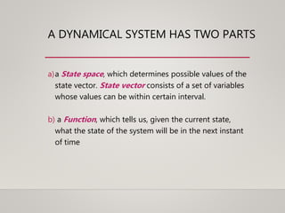
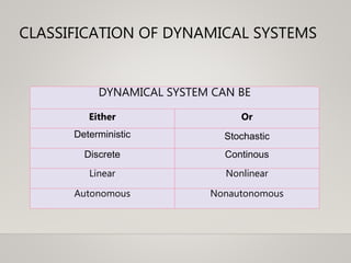
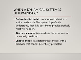
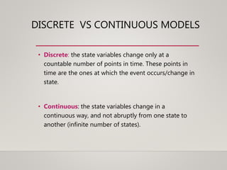
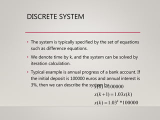
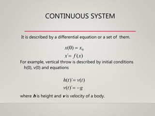
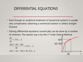
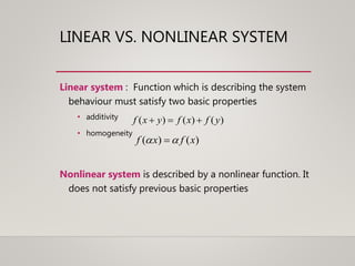
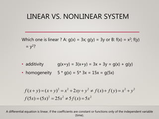
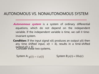
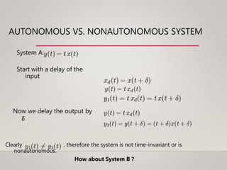
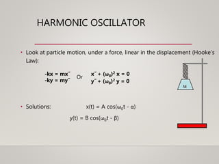
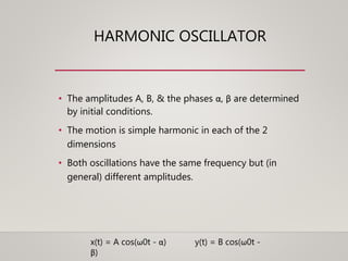
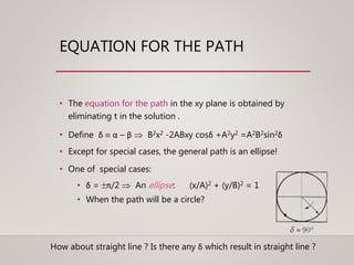
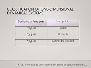
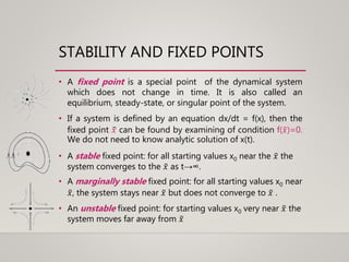
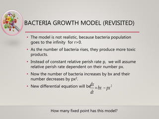
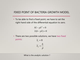
This document discusses dynamical systems. It defines a dynamical system as a system that changes over time according to fixed rules determining how its state changes from one time to the next. It then covers: - The two parts of a dynamical system: state space and function determining next state. - Classification of systems as deterministic/stochastic, discrete/continuous, linear/nonlinear, and autonomous/nonautonomous. - Examples of discrete and continuous models, differential equations, and linear vs nonlinear systems. - Terminology including phase space, phase curve, phase portrait, and attractors. - Analysis methods including fixed points, stability, and perturbation analysis. - Examples of harmonic oscillator,

1. 5. DYNAMICAL SYSTEM

2. 5.1 WHAT IS DYNAMICAL SYSTEM

3. WHAT IS A DYNAMICAL SYSTEM?
Dynamical system is a system that changes over
time according to a set of fixed rules that
determine how one state of the system moves to
another state.

4. A DYNAMICAL SYSTEM HAS TWO PARTS
a)a State space, which determines possible values of the
state vector. State vector consists of a set of variables
whose values can be within certain interval.
b) a Function, which tells us, given the current state,
what the state of the system will be in the next instant
of time

5. CLASSIFICATION OF DYNAMICAL SYSTEMS
DYNAMICAL SYSTEM CAN BE
Either Or
Deterministic Stochastic
Discrete Continous
Linear Nonlinear
Autonomous Nonautonomous

6. WHEN A DYNAMICAL SYSTEM IS
DETERMINISTIC?
• Deterministic model is one whose behavior is
entire predictable. The system is perfectly
understood, then it is possible to predict precisely
what will happen.
• Stochastic model is one whose behavior cannot
be entirely predicted.
• Chaotic model is a deterministic model with a
behavior that cannot be entirely predicted

7. DISCRETE VS CONTINUOUS MODELS
• Discrete: the state variables change only at a
countable number of points in time. These points in
time are the ones at which the event occurs/change in
state.
• Continuous: the state variables change in a
continuous way, and not abruptly from one state to
another (infinite number of states).

8. 100000*03.1)(
)(03.1)1(
100000)0(
k
kx
kxkx
x



DISCRETE SYSTEM
• The system is typically specified by the set of equations
such as difference equations.
• We denote time by k, and the system can be solved by
iteration calculation.
• Typical example is annual progress of a bank account. If
the initial deposit is 100000 euros and annual interest is
3%, then we can describe the system by

9. CONTINUOUS SYSTEM
It is described by a differential equation or a set of them.
For example, vertical throw is described by initial conditions
h(0), v(0) and equations
where h is height and v is velocity of a body.
)(´
)0( 0
xfx
xx


gtv
tvth


)´(
)()´(

10. 10
DIFFERENTIAL EQUATIONS
• Even though an analytical treatment of dynamical systems is usually
very complicated, obtaining a numerical solution is (often) straight
forward.
• Solving differential equations numerically can be done by a number
of schemes. The easiest way is by the 1st order Euler’s Method:
,..)()()(
,...)(
)()(
,...)(
xftttxtx
xf
t
ttxtx
xf
dt
dx





t
x
Δt
x(t)
x(t-Δt)

11. LINEAR VS. NONLINEAR SYSTEM
Linear system : Function which is describing the system
behaviour must satisfy two basic properties
• additivity
• homogeneity
Nonlinear system is described by a nonlinear function. It
does not satisfy previous basic properties
)()()( yfxfyxf 
)()( xfxf  

12. LINEAR VS. NONLINEAR SYSTEM
Which one is linear ? A: g(x) = 3x; g(y) = 3y or B: f(x) = x2; f(y)
= y2?
• additivity g(x+y) = 3(x+y) = 3x + 3y = g(x) + g(y)
• homogeneity 5 * g(x) = 5* 3x = 15x = g(5x)
222
22222
5)(525)5()5(
)()(2)()(
xxfxxxf
yxyfxfyxyxyxyxf


A differential equation is linear, if the coefficients are constant or functions only of the independent variable
(time).

13. AUTONOMOUS VS. NONAUTONOMOUS SYSTEM
Autonomous system is a system of ordinary differential
equations, which do not depend on the independent
variable. If the independent variable is time, we call it time-
invariant system.
Condition: If the input signal x(t) produces an output y(t) then
any time shifted input, x(t + δ), results in a time-shifted
output y(t + δ)
Consider these two systems,
System A: System B: )(10)( txty 

14. AUTONOMOUS VS. NONAUTONOMOUS SYSTEM
Clearly , therefore the system is not time-invariant or is
nonautonomous.
System A:
Start with a delay of the
input
Now we delay the output by
δ
How about System B ?

15. 5.2 DYNAMICAL SYSTEMS TERMINOLOGY

16. DYNAMICAL SYSTEMS TERMINOLOGY
• A phase space is a space in which all possible states
of a system are represented, with each possible state
of the system corresponding to one unique point in
the phase space.
• The phase space of a two-dimensional system is
called a phase plane.
• A phase curve is a plot of the solution of equations of
motion in a phase space.
• A phase portrait is a plot of single phase curve or
multiple phase curves corresponding to different
initial conditions in the same phase plane.

17. DIFFERENTIAL EQUATION OF A SYSTEMS
• Predator-Prey Relationships

18. 18
LOTKA-VOLTERRA EQUATIONS
• The Lotka-Volterra equations describe the interaction between two
species, prey vs. predators, e.g. rabbits vs. foxes.
x: number of prey
y: number of predators
α, β, γ, δ: parameters
)(
)(
xy
dt
dy
yx
dt
dx




Can you model of Predator-Prey system using Cellular Automata ?

19. 19
LOTKA-VOLTERRA EQUATIONS
• The Lotka-Volterra equations describe the interaction between two
species, prey vs. predators, e.g. rabbits vs. foxes.
Can you solve predator-prey system in the Mathematica and reproduce these
graphs?

20. HARMONIC OSCILLATOR
• Look at particle motion, under a force, linear in the displacement (Hooke’s
Law):
• Solutions: x(t) = A cos(ω0t - α)
y(t) = B cos(ω0t - β)
Or
x˝ + (ω0)2 x = 0
y˝ + (ω0)2 y = 0
-kx = mx˝
-ky = my˝

21. HARMONIC OSCILLATOR
• The amplitudes A, B, & the phases α, β are determined
by initial conditions.
• The motion is simple harmonic in each of the 2
dimensions
• Both oscillations have the same frequency but (in
general) different amplitudes.
x(t) = A cos(ω0t - α) y(t) = B cos(ω0t -
β)

22. EQUATION FOR THE PATH
• The equation for the path in the xy plane is obtained by
eliminating t in the solution .
• Define δ  α – β  B2x2 -2ABxy cosδ +A2y2 =A2B2sin2δ
• Except for special cases, the general path is an ellipse!
• One of special cases:
• δ = π/2  An ellipse: (x/A)2 + (y/B)2 = 1
• When the path will be a circle?
How about straight line ? Is there any δ which result in straight line ?

23. 5.3 DYNAMICAL SYSTEMS ANALYSIS

24. DYNAMICAL SYSTEMS ANALYSIS
How many equilibria a coin balanced on a table have
? Heads, Tails, Edge
Start on its edge, it is in equilibrium … is it stable?
… No! Small movement away (perturbation) means that coin will
end up in one of 2 different equilibria: Heads/ Tails.
Both stable as perturbation does not result in a change in state

25. Similarly, think of a ball at rest in a dark landscape. It’s either on top of a hill or
at the bottom of a valley. To find out which, push it (perturb it), and see if it
comes back. (What about flat bits?)

26. ATTRACTOR & PERTURBATION
• An attractor is a set towards which a dynamical system
evolves over time. It can be a point, a curve or more
complicated structure
• A perturbation is a small change in a physical system,
most often in a physical system at equilibrium that is
disturbed from the outside
• Each attractor has a basin of attraction which contains
all the initial conditions which will generate trajectories
joining asymptotically this attractor

27. FIXED POINTS OF 1D SYSTEMS
One dimensional system, dx/dt = f(x, t)
At a fixed point, x doesn’t change as time increases:
dx/dt = 0
So, to find fixed points, f(x, t) = 0 should be solved
Note: same procedure for finding maxima and minima

28. What are the fixed points of this system dx/dt = 6x(1 – x) ?
so either 6x = 0 => x = 0 or 1 – x = 0 => x = 1
Set:dx/dt = 0 ie: 6x(1-x) = 0
But to perturb them must have a model of the system.
Use difference equation: x(t+h) = x(t) +h dx/dt from various different
initial x’s
Perturb the points and see what happens …

29. x=0 unstable and x=1 stable.
Start from:
x = 0 + 0.01, x = 0 – 0.01,
x = 1 + 0.01, x = 1 – 0.01
….
0 0.5 1 1.5
0
0.1
0.2
0.3
0.4
0.5
0.6
0.7
0.8
0.9
1
t
x

30. CLASSIFICATION OF ONE-DIMENSIONAL
DYNAMICAL SYSTEMS
Derivative at fixed point Fixed point is
f'(a0) <0 Stable
f'(a0) >0 Unstable
f'(a0) =0 Cannot be decided
if f’(a0) = 0 it can be semi-stable from above or below or periodic …

31. STABILITY AND FIXED POINTS
• A fixed point is a special point of the dynamical system
which does not change in time. It is also called an
equilibrium, steady-state, or singular point of the system.
• If a system is defined by an equation dx/dt = f(x), then the
fixed point 𝑥 can be found by examining of condition f( 𝑥)=0.
We do not need to know analytic solution of x(t).
• A stable fixed point: for all starting values x0 near the 𝑥 the
system converges to the 𝑥 as t→∞.
• A marginally stable fixed point: for all starting values x0 near
𝑥, the system stays near 𝑥 but does not converge to 𝑥 .
• An unstable fixed point: for starting values x0 very near 𝑥 the
system moves far away from 𝑥

32. BACTERIA GROWTH MODEL
• We leave a nutritive solution and some bacteria in a
dish.
• Let b be relative rate at which the bacteria reproduce
and p be relative rate at which they die. Then the
population is growing at the rate r = b−p.
• If there are x bacteria in the dish then the rate at
which the number of bacteria is increasing is (b − p)x,
that is, dx/dt = rx.
• Solution of this equation for x(0)=x0 is
rt
extx 0)( 
Is this model
realistic?

33. BACTERIA GROWTH MODEL (REVISITED)
• The model is not realistic, because bacteria population
goes to the infinity for r>0.
• As the number of bacteria rises, they produce more toxic
products.
• Instead of constant relative perish rate p, we will assume
relative perish rate dependent on their number px.
• Now the number of bacteria increases by bx and their
number decreases by px2.
• New differential equation will be 2
pxbx
dt
dx

How many fixed point has this model?

34. FIXED POINT OF BACTERIA GROWTH MODEL
• To be able to find a fixed point, we have to set the
right-hand side of the differential equation to zero.
• There are two possible solutions, we have two fixed
points:
0)~(~
0~~ 2


xpbx
xpxb
p
b
x
x


2
1
~
0~
What is the analytic solution ?

35. FIRST FIXED POINT IS UNSTABLE
• There are no bacteria, None can be born, None can
die
• But after small contamination (perturbation) which
is smaller than b/p, the number of bacteria will
increase by dx/dt = bx-px2>0 and will never return
to the zero state.

36. THE SECOND FIXED POINT IS STABLE AND IS ALSO AN ATTRACTOR
• Second point 𝑥= b/p, at this population level, bacteria are
being born at a rate b 𝑥=b(b/p) = b2/p and are dying at a rate
p 𝑥2 = b2/p, so birth and death rates are exactly in balance.
• If the number of bacteria would be slightly increased, then
dx/dt = bx-px2<0 and would return to equilibrium.
• If the number of bacteria would be slightly decreased, then
dx/dt = bx-px2>0 and would return to equilibrium.
• Small perturbations away from 𝑥= b/p will self-correct back to
b/p.
How does the graphic solution in Mathematica look like?

37. 5.4 2D DYNAMICAL SYSTEMS

38. 2D DYNAMICAL SYSTEMS
1. Find fixed points
2. Examine stability of fixed points
3. Examine the phase plane and trajectories
),(
),(
yxgy
dt
dy
yxfx
dt
dx




Suppose we have the following system :

39. FIND FIXED POINTS
• Find fixed points as before we need to solve: f(x,y) = 0
and g(x,y) = 0 to get fixed points (x0, y0)
• Predator-prey system :
• If x=0, dy/dt = -0.4y -> y=0 for dy/dt=0 -> fixed point at
(0,0) and similarly, if y=0, dx/dt = 0 for x=0 so again, (0,0)
is fixed point.
• Other fixed point at (80, 12)
yxyy
xyxx
4.0005.0
05.06.0





40. 0 5 10 15 20 25
0
20
40
60
80
100
120
140
160
180
200
t
Populationsize
20 40 60 80 100 120 140 160 180 200
0
5
10
15
20
25
x
y
EXAMINE BEHAVIOR AT/NEAR FIXED POINTS
x and y in
phase-
plane
x and y
over time
Cyclic behaviour is fixed but system not at a fixed point: complications of higher dimensions

41. JACOBIAN MATRIX







































n
nnn
n
n
x
f
x
f
x
f
x
f
x
f
x
f
x
f
x
f
x
f
...
.........
...
...
21
2
2
2
1
2
1
2
1
1
1
J
Jacobian matrix is the matrix of all first-order partial derivatives of a
vector- or scalar-valued function with respect to another vector. This
matrix is frequently being marked as J, Df or A.
),....,,(
.
.
),....,,(
),....,,(
21
2122
2
2111
1
nnn
n
n
n
xxxfx
dt
dx
xxxfx
dt
dx
xxxfx
dt
dx






),....,,(
.
.
),....,,(
),....,,(
21
2122
2
2111
1
nnn
n
n
n
xxxfx
dt
dx
xxxfx
dt
dx
xxxfx
dt
dx







42. CLASSIFICATION OF 2-DIMENSIONAL LINEAR
212122
212111
),(
),(
dxcxxxfx
bxaxxxfx
































dc
ba
x
f
x
f
x
f
x
f
2
2
1
2
2
1
1
1
AJ
0)(0))((
0det0)det(
2










bcaddabcda
dc
ba



EA
Set of equations for 2D system
Jacobian matrix for 2D system
Calculation of eigenvalues

43. CLASSIFY FIXED POINTS
• If eigenvalues have negative real parts, x0 asymptotically
stable
• If at least one has positive real part, x0 unstable
• If eigenvalues are pure imaginary, stable or unstable
Complex numbers are made up of a real part (normal number) and an imaginary
part eg 4 + 3i where1i

44. BRIEF CLASSIFICATION OF 2D SYSTEMS

45. BACK TO EXAMPLE
• fx = 0.6 – 0.05y, fy = 0.05x, gx = 0.005y, gy = 0.005x – 0.4
• For J(0,0) eigenvalues 0.6 and –0.4 and eigenvectors (1,0) and (0,1).
Unstable (a saddle point) with main axes coordinate axes
• For J(80,12) eigenvalues are pure imaginary: need more info but will be
like a centre…. to the phase-plane!








4.00
06.0
)0,0(J 






04
6.00
)12,80(J
yxyy
xyxx
4.0005.0
05.06.0





46. QUALITATIVE BEHAVIOR
• For a dynamical system to be stable:
• The real parts of all eigenvalues must be negative.
• All eigenvalues lie in the left half complex plane.
• Terminology:
• Underdamped = spiral (some complex eigenvalue)
• Overdamped = nodal (all eigenvalues real)
• Critically damped = the boundary between.

47. Is there any classification for linear 3D systems using Eigen
values?
CLASSIFICATION OF DYNAMICAL SYSTEMS
USING JACOBIAN MATRIX

48. ATTRACTING NODE OF 2D LINEAR SYSTEMS
22
11
4xx
xx













40
01
A
Equations
Jacobian matrix
Eigenvalues
λ1= -1
λ2= -4
Eigenvectors












1
0
0
1
There is a stable fixed point, the attracting node or sink

49. SADDLE POINT
22
11
4xx
xx











40
01
A
Equations
Jacobian matrix
Eigenvalues
λ1= -1
λ2= 4
Eigenvectors












1
0
0
1
REPELLING NODE
There is an unstable fixed point for both
systems
22
11
4xx
xx




Equations
Jacobian matrix
Eigenvalues
λ1= 1
λ2= 4







40
01
A
Eigenvectors












1
0
0
1

50. 5.5 THE LORENZ SYSTEM

51. • Professor of Meteorology at the
Massachusetts Institute of
Technology
• In 1963 derived a three
dimensional system in efforts to
model long range predictions for
the weather
• The weather is complicated! A
theoretical simplification was
necessary
Edward Lorenz

52. THE LORENZ SYSTEM
D. Gulick, Encounters with Chaos, Mc-Graw Hill, Inc., New York, 1992.
• The Lorenz systems describes the motion of a fluid between two layers
at different temperature. Specifically, the fluid is heated uniformly from
below and cooled uniformly from above.
• By rising the temperature difference between the two surfaces, we
observe initially a linear temperature gradient, and then the formation of
Rayleigh-Bernard convection cells. After convection, turbulent regime is
also observed.

53. 53
LORENZ ATTRACTOR
• The Lorenz attractor defines a 3-dimensional trajectory by the
differential equations:
dx
dt
 (y  x)
dy
dt
 rx  y  xz
dz
dt
 xy  bz
σ, r, b are parameters
The most frequently used values of parameters:
δ= 10, r= 28 and β= 8/3

54. LORENZ ATTRACTOR
• When calculating this model, Lorenz encountered a
strange phenomenon. After entering slightly different
input values for two successive attempts he obtained
completely different outputs.
• This effect was later named a butterfly effect, which
should express the sensitivity to initial condition by a
metaphor that „a single flap of butterfly wings in South
America can change weather in Texas“.

55. LORENZ RESULT COMPARISON
Very slight change of initial condition results in large change in solution of th
function.

56. EQUILIBRIA
S1 = 0,0,0( )
S2 = b r -1( ), b r -1( ),r -1( )
S3 = - b r -1( ),- b r -1( ),r -1( )

57. LINEAR STABILITY OF S1
Jacobian
Eigenvalues of J l1,2 =
- s +1( )± s -1( )2
+ 4sr
2
l3 = -b
J 0,0,0( ) =
-s s 0
r -1 0
0 0 - b
é
ë
ê
ê
ê
ù
û
ú
ú
ú
What can you say about the Linear stability of S1 and parameter r

58. CHAOS
• A chaotic system is roughly defined by sensitivity to
initial conditions: infinitesimal differences in the initial
conditions of the system result in large differences in
behavior.
• Chaotic systems do not usually go out of control, but stay
within bounded operating conditions.
• Chaos provides a balance between flexibility and
stability, adaptiveness and dependability.
• Chaos lives on the edge between order and
randomness.

59. AN ATTRACTOR OF DYNAMICAL SYSTEM
• Fixed point. The system evolves towards a single state and remains
there. An example is damped pendulum or a sphere at the bottom of
a spheric bowl.
• Periodic or quasiperiodic attractor: The system evolves towards a limit
cycle. An example is undamped pendulum or a planet orbiting
around the Sun.
• Chaotic attractor: The system is very sensitive to initial conditions and
we are not able to simply predict its behavior. An example is the
Lorenz attractor.
• Strange attractor: The system is also very sensitive to initial conditions
and we are not able to simply predict its behavior, but in this case the
system has the same properties like fractals. An example is the
Mandelbrot set.

60. FRACTALS
• The fractal is a geometric shape, that has the following features:
• It is self-similar, which means, that observing the shape in various zooms results in
the same characteristic shapes (or at least approximately the same)
• It has a simple and recursive definition
• It has a fine structure at arbitrarily small scales
• It is too irregular to be easily described in traditional Euclidean geometric
language.
• It has a Hausdorff dimension of its border higher than the topological dimension
of the border.
• Topological dimension – a point has topological dimension 0, a line has topological
dimension 1, a surface has topological dimension 2, etc.
• Hausdorff dimension – if an object contains n copies of itself reduced to one k-th of the
original dimension, the Hausdorff dimension can be calculated as log(n)/log(k)
Example – a Cantor set

61. DYNAMICAL SYSTEMS
• systems live in phase space
• of low dimension, compact or open
• or of high dimension (infinite in case of PDEs)
• and develop in time
• continuous time: differential equations
• discrete time: difference equations
• the dynamical laws may be
• deterministic (no uncertainty in the laws)
• stochastic (due to fluctuations)

62. 5.6 DISCRETE DYNAMICAL SYSTEM

63. CONTINUOUS OR DISCRETE
The pendulum is a 2-dimensional continuous dynamical
system.
A Cellular Automaton or Boolean network are a discrete
dynamical system.
If there are 100 cells, then it is a 100-dim DS with a
deterministic trajectory (following all the update rules) --
strictly you need a 100-dim graph to picture it.

64. BOOLEAN NETWORK
Boolean network is
- a directed graph G(V,E)
characterized by
- the number of nodes : N
- the number of inputs per node: k
A B
C
E
D
F G

65. BOOLEAN LOGIC
Boolean models are discrete (in state and time) and deterministic.
(George Boole, 1815-1864)
Each node can assume one of two states:
on („1“) or off („0“)
Background:
Not enough information for more detailed description
Increasing complexity and computational effort for more specific models
Replacement of continuous
functions (e.g. Hill function)
by step function

66. BOOLEAN NETWORK
7
2
2
Boolean networks have
always a finite number of possible states: 2N
and, therefore, a finite number of state transitions:
A B
C
E
D
F G
N=7, 27 states, theoretically possible state transition
N
2
2

67. DYNAMICS OF BOOLEAN NETWORKS
The dynamics are described by rules:
„if input value/s at time t is/are...., then output value at t+1 is....“
A B
A(t) B(t+1)

68. BOOLEAN MODELS: TRUTH FUNCTIONS
in output
0 0 0 1 1
1 0 1 0 1
p p not p
rule 0 1 2 3
A B
B(t+1) = not (A(t))
rule 2
A(t) B(t+1)

69. STATE SPACE OF BOOLEAN
NETWORKS
State of the net: Row listing the present value of all N elements (0 or 1)
Finite number of states (2N)  as system passes along a sequence of states from
an arbitrary initial state, it must eventually re-enter a state previously passed  a
cycle
Cycle length: number of states on a re-enterant cycle of behavior
Cycle of length 1 – equilibrial state
Transient (or run-in) length: number of state between initial states and entering the
cycle
Confluent: set of states leading to or being part of a cycle

70. DYNAMICS OF BOOLEAN NETWORKS WITH K=1
Linear chainA B C D
A fixed (no input).
A(t)  B(t+1)
B(t+1)  C(t+2)
C(t+2)  D(t+3)
The system reaches a steady state after N-1 time steps.
Rules 0 and 3 not considered (since independence of input).

71. DYNAMICS OF BOOLEAN NETWORKS WITH K=1
Ring
A B
C D
A
B
Again: Rules 0 and 3 not considered (since independence of
input).
A(t+1)=B(t)
B(t+1)=A(t)
Both rule 1
A B A B A B A B
0 0 1 0 0 1 1 1
0 0 0 1 1 0 1 1
0 0 1 0 0 1 1 1
A(t+1)=not B(t)
B(t+1)=A(t)
Both rule 2
A B A B A B A B
0 0 1 0 0 1 1 1
1 0 1 1 0 0 0 1
1 1 0 1 1 0 0 0
0 1 0 0 1 1 1 0
0 0 1 0 0 1 1 1
Fixed point or
cycle of length 2
depending on
initial conditions
Cycle of length 4
independent of
initial conditions.

72. 5.7 KAUFFMAN MODEL

73. KAUFFMAN MODEL
• In 1969, Stuart Kauffman proposed using Random
Boolean Networks (RBNs) as an abstract model of
gene regulatory networks
• Each vertex represents a gene
• “on” state of a vertex indicates that the gene is
expressed
• An edge from one vertex to another implies the
the former gene regulates the later
• “0” and “1” values on edges indicate presence/
absence of activating/repressing proteins
• Boolean functions assigned to vertices represent
rules of regulatory interactions between genes

74. EXAMPLE NETWORK
Three genes X, Y, and Z
X
Y
Z
Rules
X(t+1) = X(t) and Y(t)
Y(t+1) = X(t) or Y(t)
Z(t+1) = X(t) or (not Y(t) and Z(t))
Current Next
state state
000 000
001 001
010 010
011 010
100 011
101 011
110 111
111 111
000 001 010 011
100
101 110 111

75. EXAMPLE NETWORK
000 001 010 011
100
101 110 111
X
Y
Z
- The number of accessible states is finite, .
- Cyclic trajectories are possible.
- Not every state must be approachable from every other state.
- The successor state is unique, the predecessor state is not unique.
N
2

76. RANDOM BOOLEAN NETWORKS
If the rules for updating states are unknown
 select rules randomly
N nodes ½ pN (N-1) edges
Rule 2
Rule 0
Rule 1
Rule 2

77. KAUFFMAN’S NK BOOLEAN NETWORKS
An NK automaton is an autonomous random network of N Boolean logic
elements. Each element has K inputs and one output. The signals at inputs
and outputs take binary (0 or 1) values. The Boolean elements of the
network and the connections between elements are chosen in a random
manner. There are no external inputs to the network. The number of
elements N is assumed to be large.

78. KAUFFMAN’S NK BOOLEAN NETWORKS
K connections: 22K
Boolean input functions
Nets are free of external inputs.
Once, connections and rules are selected, they remain constant and the
time evolution is deterministic.
Earlier work by Walker and Ashby (1965): same Boolean functions for all
genes:
Choice of Boolean function affects length of cycles:
“and” yields short cycles,
“exclusive or” yields cycles of immense length

79. DYNAMICS WHEN N
• Number and length of attractors of depend on k and p
kc = ½ p(1-p)
 k < kc frozen phase
 many small attractors, not sensitive to changes in structure
 k > kc chaotic phase
 few large attractors, very sensitive to changes in structure
 k = kc phase transition behavior
 n attractors of length n, not sensitive to most changes, only to
some rare ones

80. KAUFFMAN MODEL
• Gene regulatory networks of living cells are believed
to exhibit phase transition behavior, on the border
between the frozen and chaotic phases
• Kaufman has shown that if k = 2 and p = 0.5, then the
statistical features of RBNs match the characteristics of
living cells
• Number of attractors  number of cell types
• Length of attractors  cell cycle time