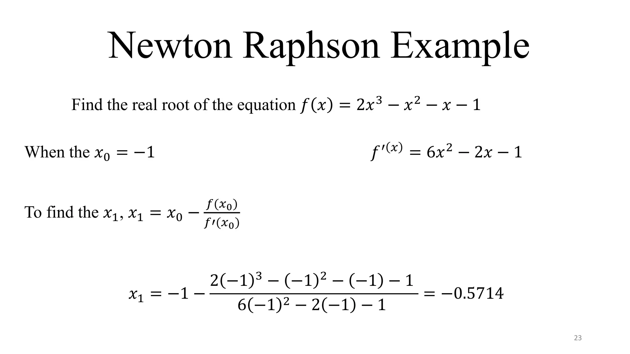
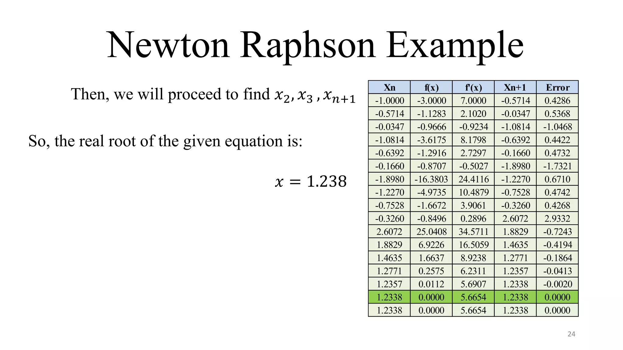
AMA 616 Advanced Mathematics
“Numerical Techniques”
Final Presentation Submitted to The Academic Department
Of the School of Science and Engineering
In Partial Fulfillment of the Requirements
For the Doctorial Degree in Mechanical Engineering
ATLANTIC INTERNATIONAL UNIVERSITY
Yasir Dhaif Mahdi Alnaseri
ID# UD67080SME76152
1
Numerical Techniques
2
Numerical Techniques
3
 Numerical Techniques are the methods involved in solving the
mathematical application models when analytical solutions do not
exist.
 Solving the partial and the ordinary differential equations by the
analytical methods are very complex and sometimes are extremely
difficult.
Numerical Techniques
After the middle of the recent century, the digital computer is
invited to be utilized for solving the complex mathematical equations
whatever its type:
 ordinary ore partial differential equations
 Linear or nonlinear
 Homogeneous or nonhomogeneous
 First-order or Higher-order
4
Numerical Techniques
Types of Equations:
1. Algebraic Equations (Ex: 𝑦 = 𝑏0 + 𝑏1 𝑥 + 𝑏2 𝑥2
+ 000 + 𝑏 𝑛 𝑥 𝑛
)
2. Transcendental Equations , Such as Logarithmic and Hyperbolic
(Ex: 𝑦 = 𝑥 sin 3𝑥 + 𝑒5𝑥)
5
Numerical Techniques Use
 Solving:
1. Linear and Nonlinear Equations
2. Differential Equations
3. Boundary Value Problems
 Evaluating:
1. Roots of Equations
2. Errors and Their Sources
3. Numerical Integration
4. Approximating Functions
6
Evaluating the Roots of Equation
There are several methods to evaluate the Roots of
Equations, such as:
1. Bi-section Method
2. Secant Method
3. Newton Raphson Method (NR)
7
Bi-section Method
 It is called the interval halving method, root-finding
method, binary method, and dichotomy method.
 It is the simplest among all the numerical methods to solve
the transcendental equations.
 It represents one of the most fundamental problems solver
in numerical analysis.
8
Bi-section Method
The Bi-section method is consists of guessing two such
numbers 𝑎 and 𝑏 , then halving the interval 𝑎 , 𝑏 and
keeping the half on which 𝑓 (𝑥) changes signs and repeating
the procedure until this interval shrinks from giving the
required accuracy for the root.
9
Bi-section Method Algorithm
An algorithm could be defined as follows:
A root for 𝑓 𝑥 = 0 , we have an error tolerance of ɛ.
Note: The absolute error in calculating the root must be less
than ɛ value.
10
Bi-section Method Procedures
1. Find TWO numbers 𝑎 and 𝑏 at which 𝑓 𝑥 has different signs.
2. Define 𝑐 =
𝑎+𝑏
2
(halving interval).
3. If 𝑏 − 𝑐 ≤ 𝜀 then accept as the root and stop.
4. If 𝑓 𝑎 𝑓(𝑐) ≤ 0 then set 𝑐 as the new 𝑏, otherwise, set 𝑐 as the new 𝑎, and
return to step 1.
11
Bi-section Method Example
𝑓 𝑥 =
1
2
𝑒 𝑥 − 3𝑥 − 3
Solution: This equation has two roots
The first root located
Between -1 and -0.5
By using the
Excel, so the approx.
Value of the first root is
-0.935546
12
Guess (a) Guess (b) Mid-point F(a) F(b) F(Mid-point) Error Test
-1 -0.5 -0.75 0.18394 -1.19673 -0.51381672 0.5 0
-1 -0.75 -0.875 0.18394 -0.51382 -0.16656899 0.25 0
-1 -0.875 -0.9375 0.18394 -0.16657 0.008302813 0.125 0
-0.9375 -0.875 -0.90625 0.008303 -0.16657 -0.07923174 0.0625 0
-0.9375 -0.90625 -0.921875 0.008303 -0.07923 -0.03548874 0.03125 0
-0.9375 -0.92188 -0.9296875 0.008303 -0.03549 -0.01359899 0.015625 0
-0.9375 -0.92969 -0.9335938 0.008303 -0.0136 -0.00264959 0.007813 0
-0.9375 -0.93359 -0.9355469 0.008303 -0.00265 0.002826239 0.003906 1
-0.93555 -0.93359 -0.9345703 0.002826 -0.00265 8.8233E-05 0.001953 1
Bi-section Method Example
𝑓 𝑥 =
1
2
𝑒 𝑥 − 3𝑥 − 3
Solution: This equation has two roots
The second root located
between 3 and 3.5
by using the
Excel, so the approx.
value of the second root
is 3.236328
13
Guess (a) Guess (b) Mid-point F(a) F(b) F(Mid-point) Error Test
3 3.5 3.25 -1.95723 3.057726 0.145169959 0.5 0
3 3.25 3.125 -1.95723 0.14517 -0.99505245 0.25 0
3.125 3.25 3.1875 -0.99505 0.14517 -0.44860889 0.125 0
3.1875 3.25 3.21875 -0.44861 0.14517 -0.15782271 0.0625 0
3.21875 3.25 3.234375 -0.15782 0.14517 -0.00787612 0.03125 0
3.234375 3.25 3.2421875 -0.00788 0.14517 0.06825645 0.015625 0
3.234375 3.242188 3.23828125 -0.00788 0.068256 0.030092928 0.007813 0
3.234375 3.238281 3.23632813 -0.00788 0.030093 0.011084142 0.003906 1
3.234375 3.236328 3.23535156 -0.00788 0.011084 0.001597951 0.001953 1
Bi-section Method Advantages
 It is always convergent.
 By increasing the number of iterations will get a more accurate root value.
 It does not require complicated calculations.
 Easy to program in the computer (Excel, Matlab, C++, etc.)
14
Bi-section Method Disadvantages
 It is generally slow.
 One guess may increase the number of the required iterations to converge the
approximate root value.
 It cannot find the root of some equations.
 It has a linear rate of convergence.
 It does not work to determine the complex roots.
15
Secant Method
 It is an open method.
 It starts with TWO initial guesses 𝑋0 & (𝑋1)
 It is suitable to determine the real roots of the non-linear equations.
16
Secant Method Procedure
1. Find the initial values 𝑋0 & (𝑋1) if it is not given.
2. Evaluate the first approximation by using the Secant method formula
𝑋2 = 𝑋1 −
𝑋1−𝑋0 ×𝐹(𝑋1)
𝐹 𝑋1 −𝐹(𝑋0)
3. To find 𝑋3, 𝑋4, 𝑋5, and 𝑋𝑛, use the Secant method formula below until reaching
the accepted error value.
𝑋𝑛 + 1 = 𝑋𝑛 −
𝑋𝑛−𝑋𝑛−1 ×𝐹(𝑋𝑛)
𝐹 𝑋𝑛 −𝐹(𝑋𝑛−1)
17
Secant Method Example
Evaluate the root of the equation 3𝑋 − 𝑒−𝑋
,
𝑋2 = 1 −
1 − 0 × 2.632121
2.632121 + 1
= 0.066636
So, the approximate root value is
𝑋 ≈ 0.257628
18
X0 X1 X2 X3 X4 X5
X 0 1.000000 0.275321 0.256499 0.257630 0.257628
F(x) -1 2.632121 0.066636 -0.004261 0.000008 0.000000
Xn Error
X2 0.275321 -0.724679
X3 0.256499 -0.018823
X4 0.257630 0.001131
X5 0.257628 -0.000002
Secant Method Advantages
 It does not need to evaluate the first derivative of the equation.
 It does not need to monitor sign change.
 The Secant method converges rapidly near a root.
19
Secant Method Disadvantages
 Sometimes, it does not converge.
 It does not give an accurate guess, so it must repeat the iteration several times
until finding a small error.
 It fails when the function is very flat.
20
Newton Raphson Method
 It called also Newton method.
 It stars with one initial guess.
 It utilizes to determine the real root of non-linear equations.
21
Newton Raphson Procedure
 Rearranging the given equation into the form 𝑓 𝑥 = 0
 Find the first derivative of 𝑓 𝑥
 Use the formula 𝑋 𝑛+1 = 𝑋 𝑛 −
𝑓(𝑥 𝑛)
𝑓′(𝑥 𝑛)
22
Newton Raphson Example
Find the real root of the equation 𝑓 𝑥 = 2𝑥3
− 𝑥2
− 𝑥 − 1
When the 𝑥0 = −1 𝑓′ 𝑥
= 6𝑥2
− 2𝑥 − 1
To find the 𝑥1, 𝑥1 = 𝑥0 −
𝑓(𝑥0)
𝑓′(𝑥0)
𝑥1 = −1 −
2 −1 3
− −1 2
− −1 − 1
6 −1 2 − 2 −1 − 1
= −0.5714
23
Newton Raphson Example
Then, we will proceed to find 𝑥2, 𝑥3 , 𝑥 𝑛+1
So, the real root of the given equation is:
𝑥 = 1.238
24
Xn f(x) f'(x) Xn+1 Error
-1.0000 -3.0000 7.0000 -0.5714 0.4286
-0.5714 -1.1283 2.1020 -0.0347 0.5368
-0.0347 -0.9666 -0.9234 -1.0814 -1.0468
-1.0814 -3.6175 8.1798 -0.6392 0.4422
-0.6392 -1.2916 2.7297 -0.1660 0.4732
-0.1660 -0.8707 -0.5027 -1.8980 -1.7321
-1.8980 -16.3803 24.4116 -1.2270 0.6710
-1.2270 -4.9735 10.4879 -0.7528 0.4742
-0.7528 -1.6672 3.9061 -0.3260 0.4268
-0.3260 -0.8496 0.2896 2.6072 2.9332
2.6072 25.0408 34.5711 1.8829 -0.7243
1.8829 6.9226 16.5059 1.4635 -0.4194
1.4635 1.6637 8.9238 1.2771 -0.1864
1.2771 0.2575 6.2311 1.2357 -0.0413
1.2357 0.0112 5.6907 1.2338 -0.0020
1.2338 0.0000 5.6654 1.2338 0.0000
1.2338 0.0000 5.6654 1.2338 0.0000
Newton Raphson Advantage
 By each iteration, the error value decreases rapidly.
 Compare with Bisection and Secant methods, the Newton Raphson method is
very fast.
25
Newton Raphson Disadvantage
 The insufficient guess of the 𝑥0 value my cause fail to converge.
 Each iteration of this method requires two functions evaluations.
26

Numerical Techniques

  • 1.
    AMA 616 AdvancedMathematics “Numerical Techniques” Final Presentation Submitted to The Academic Department Of the School of Science and Engineering In Partial Fulfillment of the Requirements For the Doctorial Degree in Mechanical Engineering ATLANTIC INTERNATIONAL UNIVERSITY Yasir Dhaif Mahdi Alnaseri ID# UD67080SME76152 1
  • 2.
  • 3.
    Numerical Techniques 3  NumericalTechniques are the methods involved in solving the mathematical application models when analytical solutions do not exist.  Solving the partial and the ordinary differential equations by the analytical methods are very complex and sometimes are extremely difficult.
  • 4.
    Numerical Techniques After themiddle of the recent century, the digital computer is invited to be utilized for solving the complex mathematical equations whatever its type:  ordinary ore partial differential equations  Linear or nonlinear  Homogeneous or nonhomogeneous  First-order or Higher-order 4
  • 5.
    Numerical Techniques Types ofEquations: 1. Algebraic Equations (Ex: 𝑦 = 𝑏0 + 𝑏1 𝑥 + 𝑏2 𝑥2 + 000 + 𝑏 𝑛 𝑥 𝑛 ) 2. Transcendental Equations , Such as Logarithmic and Hyperbolic (Ex: 𝑦 = 𝑥 sin 3𝑥 + 𝑒5𝑥) 5
  • 6.
    Numerical Techniques Use Solving: 1. Linear and Nonlinear Equations 2. Differential Equations 3. Boundary Value Problems  Evaluating: 1. Roots of Equations 2. Errors and Their Sources 3. Numerical Integration 4. Approximating Functions 6
  • 7.
    Evaluating the Rootsof Equation There are several methods to evaluate the Roots of Equations, such as: 1. Bi-section Method 2. Secant Method 3. Newton Raphson Method (NR) 7
  • 8.
    Bi-section Method  Itis called the interval halving method, root-finding method, binary method, and dichotomy method.  It is the simplest among all the numerical methods to solve the transcendental equations.  It represents one of the most fundamental problems solver in numerical analysis. 8
  • 9.
    Bi-section Method The Bi-sectionmethod is consists of guessing two such numbers 𝑎 and 𝑏 , then halving the interval 𝑎 , 𝑏 and keeping the half on which 𝑓 (𝑥) changes signs and repeating the procedure until this interval shrinks from giving the required accuracy for the root. 9
  • 10.
    Bi-section Method Algorithm Analgorithm could be defined as follows: A root for 𝑓 𝑥 = 0 , we have an error tolerance of ɛ. Note: The absolute error in calculating the root must be less than ɛ value. 10
  • 11.
    Bi-section Method Procedures 1.Find TWO numbers 𝑎 and 𝑏 at which 𝑓 𝑥 has different signs. 2. Define 𝑐 = 𝑎+𝑏 2 (halving interval). 3. If 𝑏 − 𝑐 ≤ 𝜀 then accept as the root and stop. 4. If 𝑓 𝑎 𝑓(𝑐) ≤ 0 then set 𝑐 as the new 𝑏, otherwise, set 𝑐 as the new 𝑎, and return to step 1. 11
  • 12.
    Bi-section Method Example 𝑓𝑥 = 1 2 𝑒 𝑥 − 3𝑥 − 3 Solution: This equation has two roots The first root located Between -1 and -0.5 By using the Excel, so the approx. Value of the first root is -0.935546 12 Guess (a) Guess (b) Mid-point F(a) F(b) F(Mid-point) Error Test -1 -0.5 -0.75 0.18394 -1.19673 -0.51381672 0.5 0 -1 -0.75 -0.875 0.18394 -0.51382 -0.16656899 0.25 0 -1 -0.875 -0.9375 0.18394 -0.16657 0.008302813 0.125 0 -0.9375 -0.875 -0.90625 0.008303 -0.16657 -0.07923174 0.0625 0 -0.9375 -0.90625 -0.921875 0.008303 -0.07923 -0.03548874 0.03125 0 -0.9375 -0.92188 -0.9296875 0.008303 -0.03549 -0.01359899 0.015625 0 -0.9375 -0.92969 -0.9335938 0.008303 -0.0136 -0.00264959 0.007813 0 -0.9375 -0.93359 -0.9355469 0.008303 -0.00265 0.002826239 0.003906 1 -0.93555 -0.93359 -0.9345703 0.002826 -0.00265 8.8233E-05 0.001953 1
  • 13.
    Bi-section Method Example 𝑓𝑥 = 1 2 𝑒 𝑥 − 3𝑥 − 3 Solution: This equation has two roots The second root located between 3 and 3.5 by using the Excel, so the approx. value of the second root is 3.236328 13 Guess (a) Guess (b) Mid-point F(a) F(b) F(Mid-point) Error Test 3 3.5 3.25 -1.95723 3.057726 0.145169959 0.5 0 3 3.25 3.125 -1.95723 0.14517 -0.99505245 0.25 0 3.125 3.25 3.1875 -0.99505 0.14517 -0.44860889 0.125 0 3.1875 3.25 3.21875 -0.44861 0.14517 -0.15782271 0.0625 0 3.21875 3.25 3.234375 -0.15782 0.14517 -0.00787612 0.03125 0 3.234375 3.25 3.2421875 -0.00788 0.14517 0.06825645 0.015625 0 3.234375 3.242188 3.23828125 -0.00788 0.068256 0.030092928 0.007813 0 3.234375 3.238281 3.23632813 -0.00788 0.030093 0.011084142 0.003906 1 3.234375 3.236328 3.23535156 -0.00788 0.011084 0.001597951 0.001953 1
  • 14.
    Bi-section Method Advantages It is always convergent.  By increasing the number of iterations will get a more accurate root value.  It does not require complicated calculations.  Easy to program in the computer (Excel, Matlab, C++, etc.) 14
  • 15.
    Bi-section Method Disadvantages It is generally slow.  One guess may increase the number of the required iterations to converge the approximate root value.  It cannot find the root of some equations.  It has a linear rate of convergence.  It does not work to determine the complex roots. 15
  • 16.
    Secant Method  Itis an open method.  It starts with TWO initial guesses 𝑋0 & (𝑋1)  It is suitable to determine the real roots of the non-linear equations. 16
  • 17.
    Secant Method Procedure 1.Find the initial values 𝑋0 & (𝑋1) if it is not given. 2. Evaluate the first approximation by using the Secant method formula 𝑋2 = 𝑋1 − 𝑋1−𝑋0 ×𝐹(𝑋1) 𝐹 𝑋1 −𝐹(𝑋0) 3. To find 𝑋3, 𝑋4, 𝑋5, and 𝑋𝑛, use the Secant method formula below until reaching the accepted error value. 𝑋𝑛 + 1 = 𝑋𝑛 − 𝑋𝑛−𝑋𝑛−1 ×𝐹(𝑋𝑛) 𝐹 𝑋𝑛 −𝐹(𝑋𝑛−1) 17
  • 18.
    Secant Method Example Evaluatethe root of the equation 3𝑋 − 𝑒−𝑋 , 𝑋2 = 1 − 1 − 0 × 2.632121 2.632121 + 1 = 0.066636 So, the approximate root value is 𝑋 ≈ 0.257628 18 X0 X1 X2 X3 X4 X5 X 0 1.000000 0.275321 0.256499 0.257630 0.257628 F(x) -1 2.632121 0.066636 -0.004261 0.000008 0.000000 Xn Error X2 0.275321 -0.724679 X3 0.256499 -0.018823 X4 0.257630 0.001131 X5 0.257628 -0.000002
  • 19.
    Secant Method Advantages It does not need to evaluate the first derivative of the equation.  It does not need to monitor sign change.  The Secant method converges rapidly near a root. 19
  • 20.
    Secant Method Disadvantages Sometimes, it does not converge.  It does not give an accurate guess, so it must repeat the iteration several times until finding a small error.  It fails when the function is very flat. 20
  • 21.
    Newton Raphson Method It called also Newton method.  It stars with one initial guess.  It utilizes to determine the real root of non-linear equations. 21
  • 22.
    Newton Raphson Procedure Rearranging the given equation into the form 𝑓 𝑥 = 0  Find the first derivative of 𝑓 𝑥  Use the formula 𝑋 𝑛+1 = 𝑋 𝑛 − 𝑓(𝑥 𝑛) 𝑓′(𝑥 𝑛) 22
  • 23.
    Newton Raphson Example Findthe real root of the equation 𝑓 𝑥 = 2𝑥3 − 𝑥2 − 𝑥 − 1 When the 𝑥0 = −1 𝑓′ 𝑥 = 6𝑥2 − 2𝑥 − 1 To find the 𝑥1, 𝑥1 = 𝑥0 − 𝑓(𝑥0) 𝑓′(𝑥0) 𝑥1 = −1 − 2 −1 3 − −1 2 − −1 − 1 6 −1 2 − 2 −1 − 1 = −0.5714 23
  • 24.
    Newton Raphson Example Then,we will proceed to find 𝑥2, 𝑥3 , 𝑥 𝑛+1 So, the real root of the given equation is: 𝑥 = 1.238 24 Xn f(x) f'(x) Xn+1 Error -1.0000 -3.0000 7.0000 -0.5714 0.4286 -0.5714 -1.1283 2.1020 -0.0347 0.5368 -0.0347 -0.9666 -0.9234 -1.0814 -1.0468 -1.0814 -3.6175 8.1798 -0.6392 0.4422 -0.6392 -1.2916 2.7297 -0.1660 0.4732 -0.1660 -0.8707 -0.5027 -1.8980 -1.7321 -1.8980 -16.3803 24.4116 -1.2270 0.6710 -1.2270 -4.9735 10.4879 -0.7528 0.4742 -0.7528 -1.6672 3.9061 -0.3260 0.4268 -0.3260 -0.8496 0.2896 2.6072 2.9332 2.6072 25.0408 34.5711 1.8829 -0.7243 1.8829 6.9226 16.5059 1.4635 -0.4194 1.4635 1.6637 8.9238 1.2771 -0.1864 1.2771 0.2575 6.2311 1.2357 -0.0413 1.2357 0.0112 5.6907 1.2338 -0.0020 1.2338 0.0000 5.6654 1.2338 0.0000 1.2338 0.0000 5.6654 1.2338 0.0000
  • 25.
    Newton Raphson Advantage By each iteration, the error value decreases rapidly.  Compare with Bisection and Secant methods, the Newton Raphson method is very fast. 25
  • 26.
    Newton Raphson Disadvantage The insufficient guess of the 𝑥0 value my cause fail to converge.  Each iteration of this method requires two functions evaluations. 26