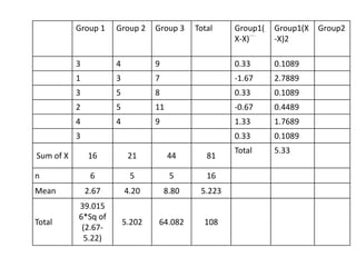
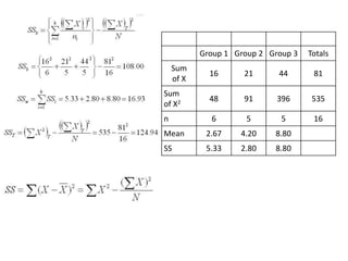
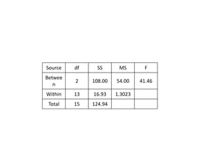
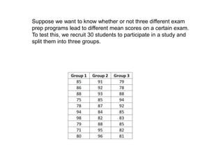
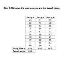
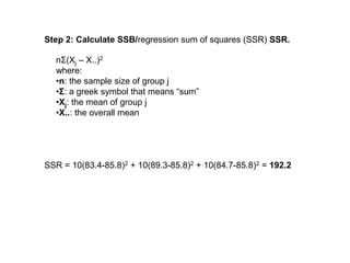
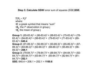
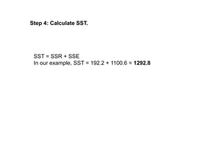
Analysis of variance (ANOVA) is a statistical technique used to compare the means of three or more groups. It compares the variance between groups with the variance within groups to determine if the population means are significantly different. The key assumptions of ANOVA are independence, normality, and homogeneity of variances. A one-way ANOVA involves one independent variable with multiple levels or groups, and compares the group means to the overall mean to calculate an F-ratio statistic. If the F-ratio exceeds a critical value, then the null hypothesis that the group means are equal can be rejected.

1. Analysis of Variance (ANOVA) is a parametric statistical technique used to compare
datasets.
This technique was invented by R.A. Fisher, and is thus often referred to as Fisher’s
ANOVA, as well.
It is similar in application to techniques such as t-test and z-test, in that it is used to
compare means and the relative variance between them.
However, analysis of variance (ANOVA) is best applied where more than 2 populations
or samples are meant to be compared.

2. The use of this parametric statistical technique involves certain key assumptions,
including the following:
1. Independence of case: Independence of case assumption means that the case of the
dependent variable should be independent or the sample should be selected randomly.
There should not be any pattern in the selection of the sample.
2. Normality: Distribution of each group should be normal. The Kolmogorov-Smirnov or
the Shapiro-Wilk test may be used to confirm normality of the group.
3. Homogeneity: Homogeneity means variance between the groups should be the
same. Levene’s test is used to test the homogeneity between groups.
If particular data follows the above assumptions, then the analysis of variance (ANOVA) is
the best technique to compare the means of two, or more, populations.

3. Analysis of variance (ANOVA) has three types:
One way analysis: When we are comparing more than three groups based on
one factor variable, then it said to be one way analysis of variance (ANOVA).
For example, if we want to compare whether or not the mean output of three
workers is the same based on the working hours of the three workers.
Two way analysis: When factor variables are two, then it is said to be two way
analysis of variance (ANOVA). For example, based on working condition and
working hours, we can compare whether or not the mean output of three
workers is the same.
K-way analysis: When factor variables are k, then it is said to be the k-way
analysis of variance (ANOVA).

4. Assumptions for Two Way ANOVA
1. The population must be close to a normal distribution.
2. Samples must be independent.
3. Population variances must be equal.
4. Groups must have equal sample sizes.

5. Key terms and concepts:
Sum of square between groups: For the sum of the square between groups, we
calculate the individual means of the group, then we take the deviation from the
individual mean for each group. And finally, we will take the sum of all groups
after the square of the individual group.
Sum of squares within group: In order to get the sum of squares within a group,
we calculate the grand mean for all groups and then take the deviation from the
individual group. The sum of all groups will be done after the square of the
deviation.
F –ratio: To calculate the F-ratio, the sum of the squares between groups will
be divided by the sum of the square within a group.

6. Degree of freedom: To calculate the degree of freedom between the sums of the
squares group, we will subtract one from the number of groups. The sum of the square
within the group’s degree of freedom will be calculated by subtracting the number of
groups from the total observation.
BSS df = (g-1) for BSS is between the sum of squares, where g is the group, and df is the
degree of freedom.
WSS df = (N-g) for WSS within the sum of squares, where N is the total sample size.
Significance: At a predetermine level of significance (usually at 5%), we will compare
and calculate the value with the critical table value. Today, however, computers can
automatically calculate the probability value for F-ratio. If p-value is lesser than the
predetermined significance level, then group means will be different. Or, if the p-value
is greater than the predetermined significance level, we can say that there is no
difference between the groups’ mean.

7. Step 1: Calculate the Mean
Step 2: Setup the null and alternate hypothesis
Step 3: Calculate the Sum of Squares
Step 4: Calculate the Degrees of Freedom
Step 5: Calculate the Mean Squares
Step 6: Calculate the F Statistic
Step 7: Look up statistical Table and state your conclusion
The hypotheses of interest in an ANOVA are as follows:
H0: μ1 = μ2 = μ3 ... = μk
H1: Means are not all equal.
where k = the number of independent comparison groups.

8. Compute a one-way ANOVA for data from three independent groups.
The raw data for the 16 subjects are listed below.
Note that this is a between-subjects design, so different people appear in
each group.
Group 1 Group 2 Group 3
3 4 9
1 3 7
3 5 8
2 5 11
4 4 9
3
Here are the raw data from the three groups (6 people in Group 1, and 5 each
in Groups 2 and 3).

9. Group 1 Group 2 Group 3 Total Group1(
X-X)
Group1(X
-X)2
Group2
3 4 9 0.33 0.1089
1 3 7 -1.67 2.7889
3 5 8 0.33 0.1089
2 5 11 -0.67 0.4489
4 4 9 1.33 1.7689
3 0.33 0.1089
Sum of X 16 21 44 81
Total 5.33
n 6 5 5 16
Mean 2.67 4.20 8.80 5.223
Total
39.015
6*Sq of
(2.67-
5.22)
5.202 64.082 108

10. Group 1 Group 2 Group 3 Totals
Sum
of X
16 21 44 81
Sum
of X2 48 91 396 535
n 6 5 5 16
Mean 2.67 4.20 8.80
SS 5.33 2.80 8.80

11. Source df SS MS F
Betwee
n
2 108.00 54.00 41.46
Within 13 16.93 1.3023
Total 15 124.94

12. Suppose we want to know whether or not three different exam
prep programs lead to different mean scores on a certain exam.
To test this, we recruit 30 students to participate in a study and
split them into three groups.

13. Step 1: Calculate the group means and the overall mean.

14. Step 2: Calculate SSB/regression sum of squares (SSR) SSR.
nΣ(Xj – X..)2
where:
•n: the sample size of group j
•Σ: a greek symbol that means “sum”
•Xj: the mean of group j
•X..: the overall mean
SSR = 10(83.4-85.8)2 + 10(89.3-85.8)2 + 10(84.7-85.8)2 = 192.2

15. Step 3: Calculate SSW/ error sum of squares (SSE)SSE.
Σ(Xij – Xj)2
where:
•Σ: a greek symbol that means “sum”
•Xij: the ith observation in group j
•Xj: the mean of group j
Group 1: (85-83.4)2 + (86-83.4)2 + (88-83.4)2 + (75-83.4)2 + (78-
83.4)2 + (94-83.4)2 + (98-83.4)2 + (79-83.4)2 + (71-83.4)2 + (80-
83.4)2 = 640.4
Group 2: (91-89.3)2 + (92-89.3)2 + (93-89.3)2 + (85-89.3)2 + (87-
89.3)2 + (84-89.3)2 + (82-89.3)2 + (88-89.3)2 + (95-89.3)2 + (96-
89.3)2 = 208.1
Group 3: (79-84.7)2 + (78-84.7)2 + (88-84.7)2 + (94-84.7)2 + (92-
84.7)2 + (85-84.7)2 + (83-84.7)2 + (85-84.7)2 + (82-84.7)2 + (81-
84.7)2 = 252.1
SSE: 640.4 + 208.1 + 252.1 = 1100.6

16. Step 4: Calculate SST.
SST = SSR + SSE
In our example, SST = 192.2 + 1100.6 = 1292.8

17. Step 5: Fill in the ANOVA table.
Source
Sum of
Squares (SS)
df
Mean Squares
(MS)
F
Treatment 192.2 2 96.1 2.358
Error 1100.6 27 40.8
Total 1292.8 29
•df treatment: k-1 = 3-1 = 2
•df error: n-k = 30-3 = 27
•df total: n-1 = 30-1 = 29
•MS treatment: SST / df treatment = 192.2 / 2 = 96.1
•MS error: SSE / df error = 1100.6 / 27 = 40.8
•F: MS treatment / MS error = 96.1 / 40.8 = 2.358
Note: n = total observations, k = number of groups

18. Step 6: Interpret the results.
The F test statistic for this one-way ANOVA is 2.358. To determine if this is
a statistically significant result, we must compare this to the F critical value
found in the F distribution table with the following values:
•α (significance level) = 0.05
•DF1 (numerator degrees of freedom) = df treatment = 2
•DF2 (denominator degrees of freedom) = df error = 27
We find that the F critical value is 3.3541.
Since the F test statistic in the ANOVA table is less than the F critical value
in the F distribution table, we fail to reject the null hypothesis. This
means we don’t have sufficient evidence to say that there is a statistically
significant difference between the mean exam scores of the three groups.