easy explaination of biostat ANOVA

1. ANOVA
1

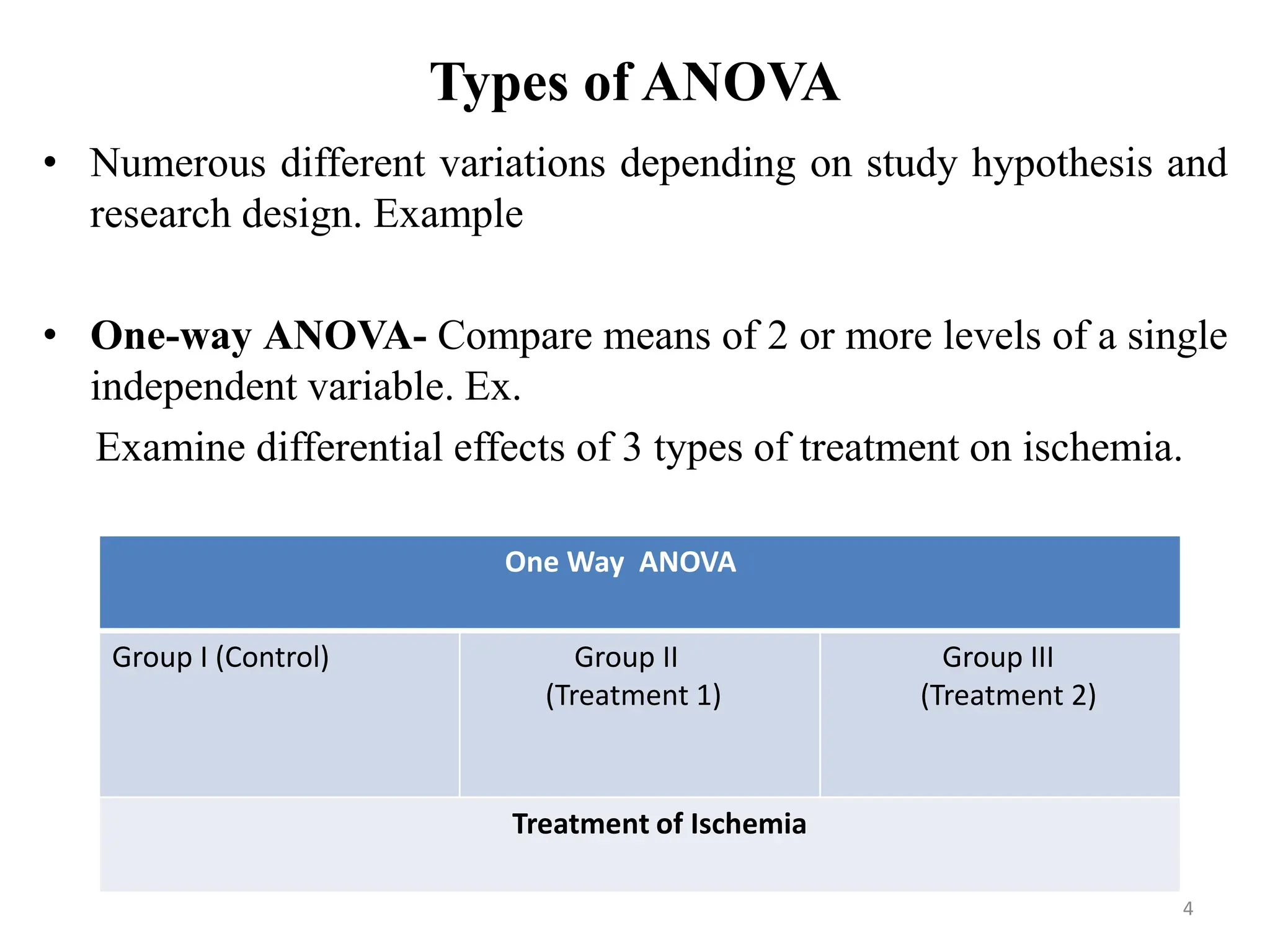
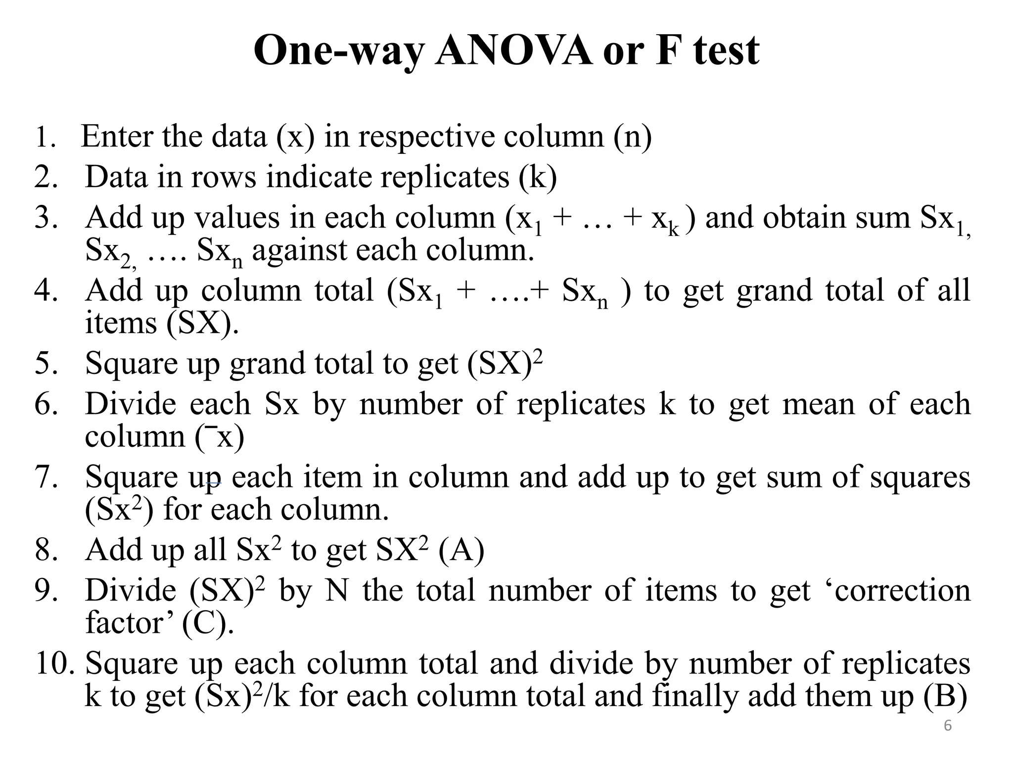
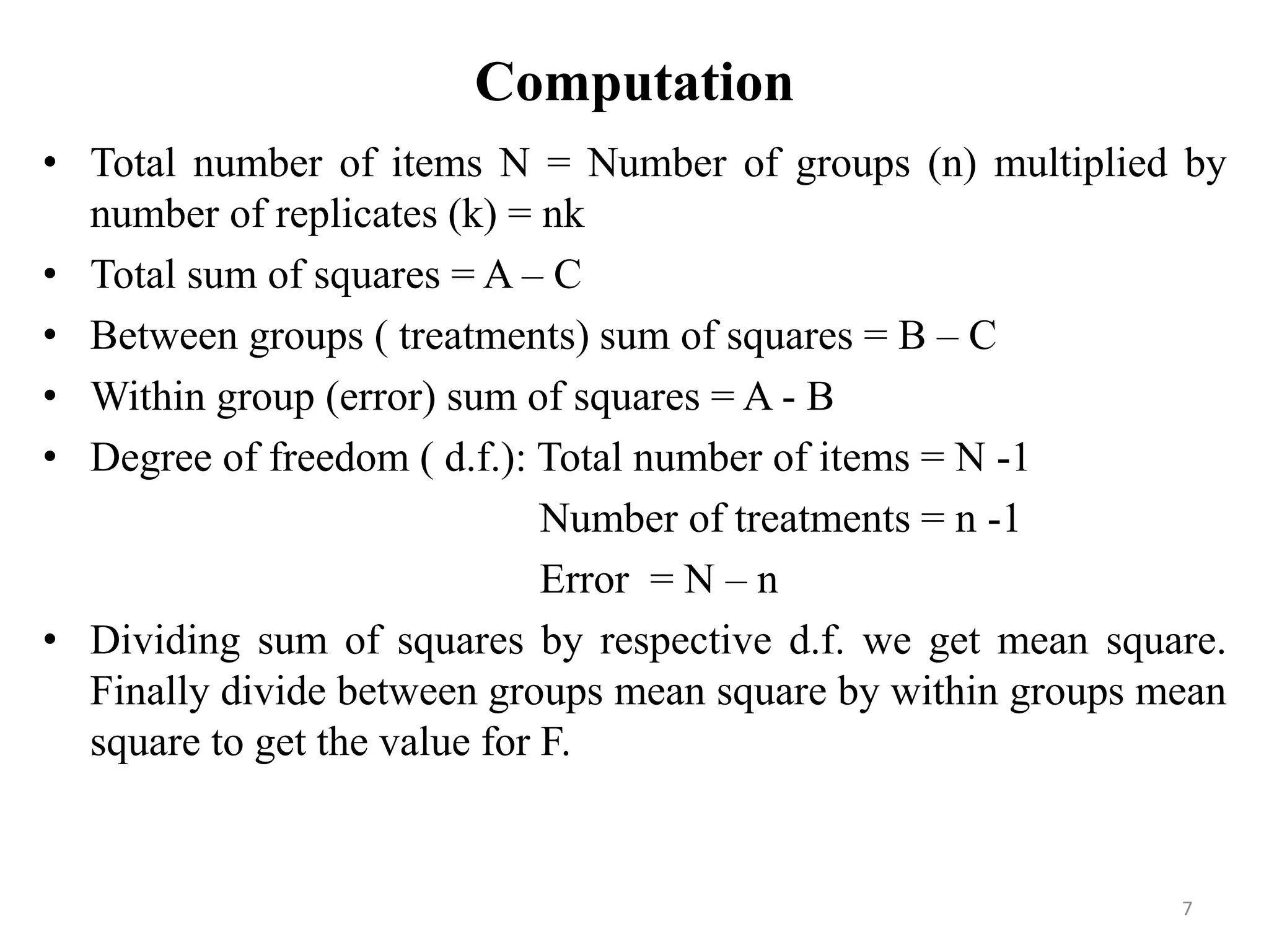
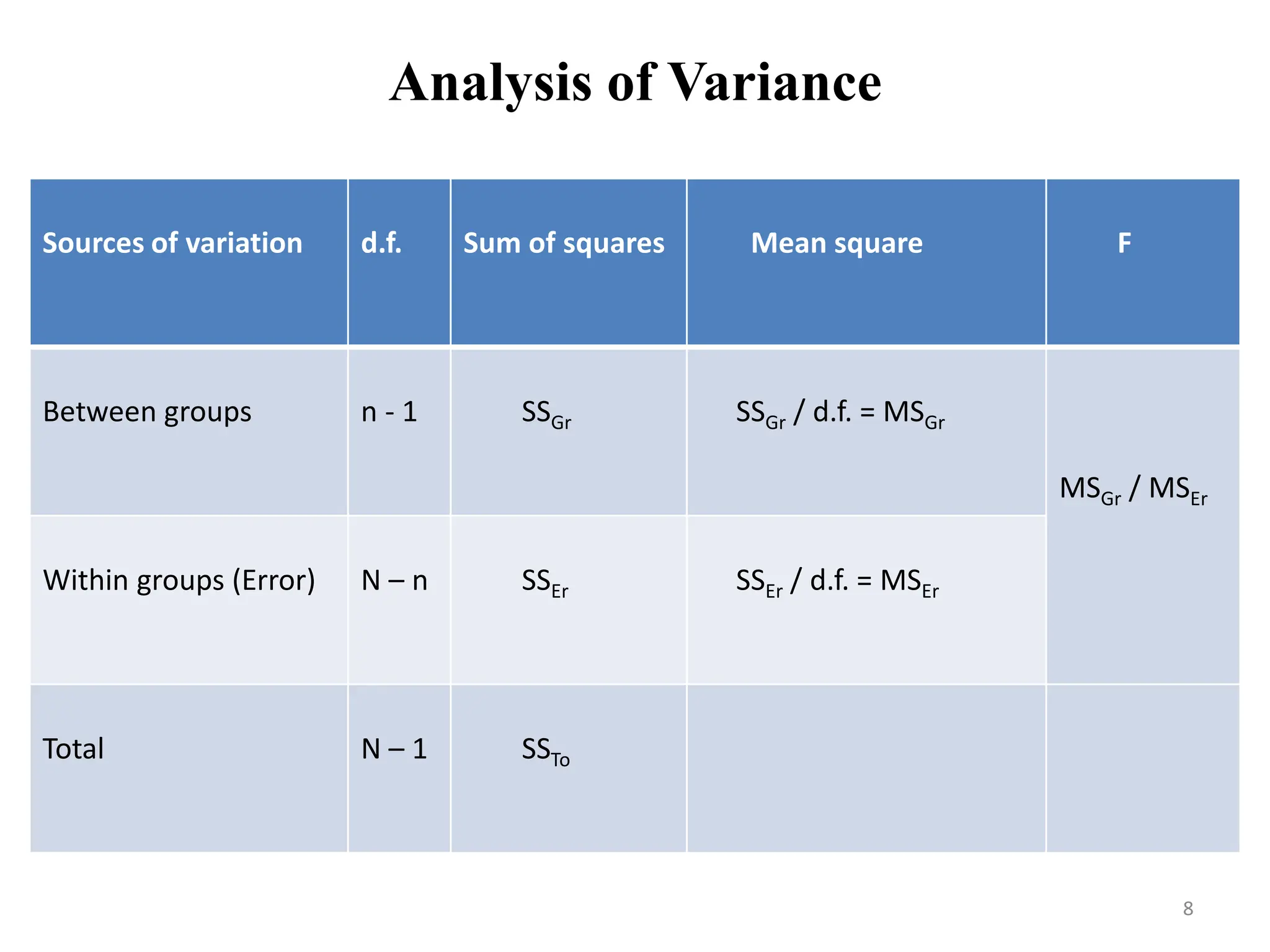
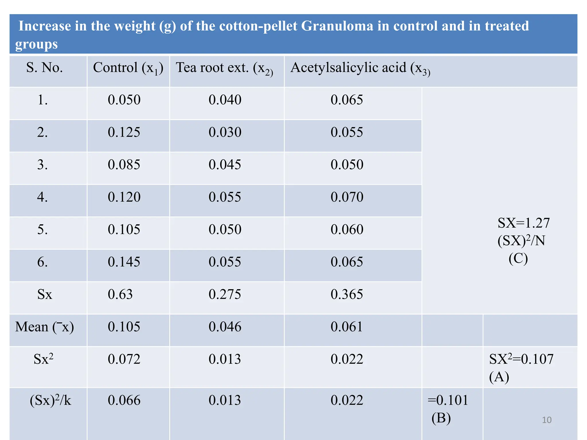
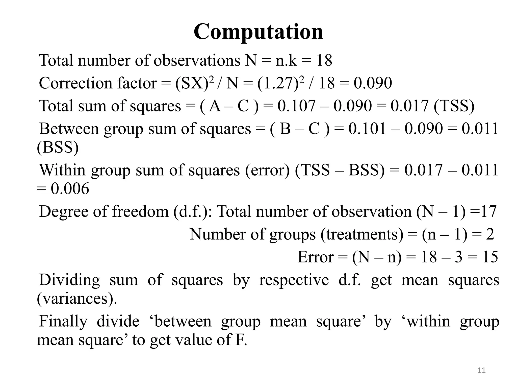
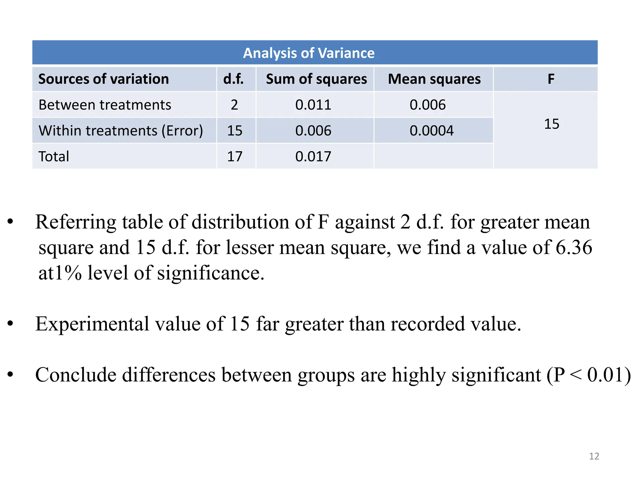
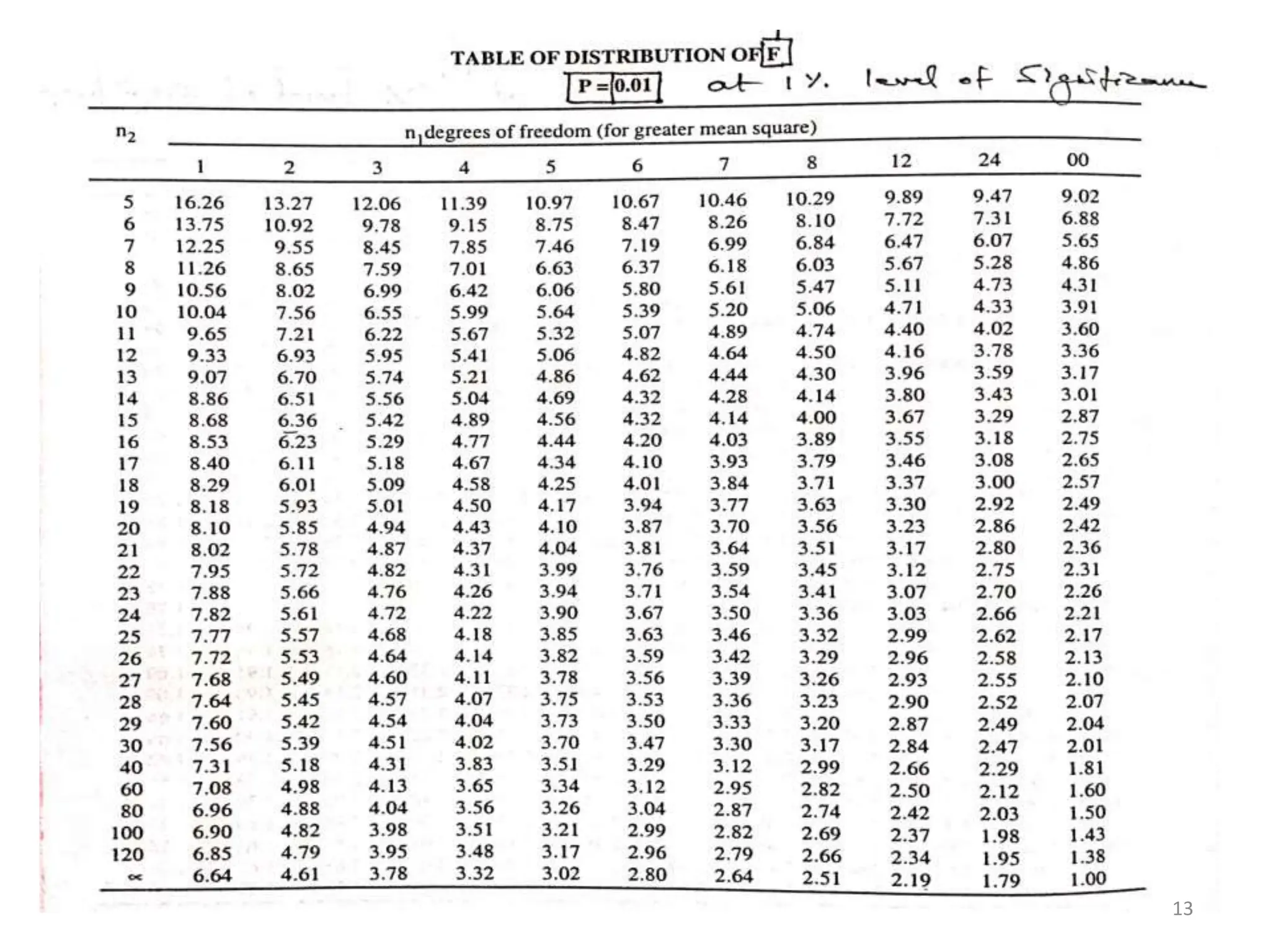
2. Analysis of Variance (ANOVA)
• Extension of t-test, major difference- it compares means across
more than 2 groups or conditions, t-test- a special case of ANOVA.
• Analysing 2 groups by ANOVA give same results as with a t-test.
• Same data analysed by series of t-test to examine difference
between more than 2 groups, not only less efficient, add
experimental error (Type 1 error).
• ANOVA works by comparing differences between group means
rather than difference between group variances, “Analysis of
variance” comes from the procedure which uses variance to decide
means different or not.
2

3. • Compares variations (variance) between groups with those within
groups. If ‘between’ and ‘within’ variances approximately of same
size- no significant difference between group means. Other hand
comparative larger ‘between’ variance indicate significant
difference between them.
• Assumption similar to t-test- all sample groups have similar
variances.
3

4. Types of ANOVA
• Numerous different variations depending on study hypothesis and
research design. Example
• One-way ANOVA- Compare means of 2 or more levels of a single
independent variable. Ex.
Examine differential effects of 3 types of treatment on ischemia.
One Way ANOVA
Group I (Control) Group II
(Treatment 1)
Group III
(Treatment 2)
Treatment of Ischemia
4

5. • Multifactor ANOVA- used when study involves 2 or more
independent variables. Ex.
Factorial design of 2, 3 to examine effectiveness of different
treatments (Factor 1) and high and low fat diet in reducing
symptoms of hypertension (Factor-2).
• Multiple analysis of variance ( MANOVA)- used when there
are 2 or more dependent variables that are generally related in
some way. Ex.
Considering above example measuring effects of different
treatments, with or without exercise, on hypertension measured
in several different ways.
Though can conduct separate ANOVA for each of these
outcomes, MANOVA provides more efficient and more
informative way of analyzing the data.
5

6. One-way ANOVA or F test
1. Enter the data (x) in respective column (n)
2. Data in rows indicate replicates (k)
3. Add up values in each column (x1 + … + xk ) and obtain sum Sx1,
Sx2, …. Sxn against each column.
4. Add up column total (Sx1 + ….+ Sxn ) to get grand total of all
items (SX).
5. Square up grand total to get (SX)2
6. Divide each Sx by number of replicates k to get mean of each
column (‾x)
7. Square up each item in column and add up to get sum of squares
(Sx2) for each column.
8. Add up all Sx2 to get SX2 (A)
9. Divide (SX)2 by N the total number of items to get ‘correction
factor’ (C).
10. Square up each column total and divide by number of replicates
k to get (Sx)2/k for each column total and finally add them up (B)
6

7. Computation
• Total number of items N = Number of groups (n) multiplied by
number of replicates (k) = nk
• Total sum of squares = A – C
• Between groups ( treatments) sum of squares = B – C
• Within group (error) sum of squares = A - B
• Degree of freedom ( d.f.): Total number of items = N -1
Number of treatments = n -1
Error = N – n
• Dividing sum of squares by respective d.f. we get mean square.
Finally divide between groups mean square by within groups mean
square to get the value for F.
7

8. Analysis of Variance
Sources of variation d.f. Sum of squares Mean square F
Between groups n - 1 SSGr SSGr / d.f. = MSGr
MSGr / MSEr
Within groups (Error) N – n SSEr SSEr / d.f. = MSEr
Total N – 1 SSTo
8

9. • Example: 3 groups of 6 rats each were assigned 3 treatments, i.e.
control, tea root extract and acetylsalicylic acid to compare their
effect on the weight of the cotton pellet granuloma. The aim of
study was to find whether there was any significant difference
between 3 groups of treatment.
9

10. Increase in the weight (g) of the cotton-pellet Granuloma in control and in treated
groups
S. No. Control (x1) Tea root ext. (x2) Acetylsalicylic acid (x3)
1. 0.050 0.040 0.065
SX=1.27
(SX)2/N
(C)
2. 0.125 0.030 0.055
3. 0.085 0.045 0.050
4. 0.120 0.055 0.070
5. 0.105 0.050 0.060
6. 0.145 0.055 0.065
Sx 0.63 0.275 0.365
Mean (‾x) 0.105 0.046 0.061
Sx2 0.072 0.013 0.022 SX2=0.107
(A)
(Sx)2/k 0.066 0.013 0.022 =0.101
(B) 10

11. Computation
Total number of observations N = n.k = 18
Correction factor = (SX)2 / N = (1.27)2 / 18 = 0.090
Total sum of squares = ( A – C ) = 0.107 – 0.090 = 0.017 (TSS)
Between group sum of squares = ( B – C ) = 0.101 – 0.090 = 0.011
(BSS)
Within group sum of squares (error) (TSS – BSS) = 0.017 – 0.011
= 0.006
Degree of freedom (d.f.): Total number of observation (N – 1) =17
Number of groups (treatments) = (n – 1) = 2
Error = (N – n) = 18 – 3 = 15
Dividing sum of squares by respective d.f. get mean squares
(variances).
Finally divide ‘between group mean square’ by ‘within group
mean square’ to get value of F.
11

12. Analysis of Variance
Sources of variation d.f. Sum of squares Mean squares F
Between treatments 2 0.011 0.006
15
Within treatments (Error) 15 0.006 0.0004
Total 17 0.017
• Referring table of distribution of F against 2 d.f. for greater mean
square and 15 d.f. for lesser mean square, we find a value of 6.36
at1% level of significance.
• Experimental value of 15 far greater than recorded value.
• Conclude differences between groups are highly significant (P < 0.01)
12

13. 13

14. Conclusion
• ANOVA compares variance of 2 or more samples, is most
elegant, powerful and useful technique by which total variation in
set of data reduced to components associated with possible source
of variability.
• F test is relatively easier to perform than t test.
• It is, however upto investigator to select the test of choice.
14

15. Thank You
15