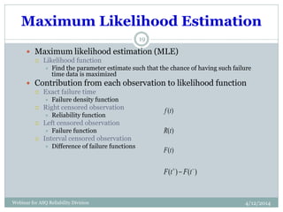
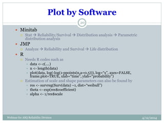
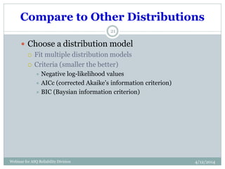
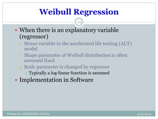
An introduction to weibull analysis

An Introduction to Weibull
Analysis (威布尔分析引论)
Rong Pan
©2014 ASQ
http://www.asqrd.org

RONG PA N
ASSOCIATE PROFESSOR
A RIZONA ST A T E U NIVERSIT Y
EM A IL: RONG.PA N@ A SU .EDU
An Introduction to Weibull
Analysis

Outlines
4/12/2014Webinar for ASQ Reliability Division
3
 Objectives
 To understand Weibull distribution
 To be able to use Weibull plot for failure time analysis and
diagnosis
 To be able to use software to do data analysis
 Organization
 Distribution model
 Parameter estimation
 Regression analysis

A Little Bit of History
4
 Waloddi Weibull (1887-1979)
 Invented Weibull distribution in 1937
 Publication in 1951
 A statistical distribution function of wide
applicability, Journal of Mechanics, ASME,
September 1951, pp. 293-297.
 Was professor at the Royal Institute of
Technology, Sweden
 Research funded by U.S. Air Force

Weibull Distribution
5
 A typical Weibull distribution function has two
parameters
 Scale parameter (characteristic life)
 Shape parameter
 A different parameterization
 Intrinsic failure rate
 Common in survival analysis
 3-parameter Weibull distribution
 Mean time to failure
 Percentile of a distribution
 “B” life or “L” life




 














t
e
t
tf
1
)(
.0,,0,1)( 










tetF
t

t
etF 
1)(








 


t
etF 1)(
)/11(  MTTF

Functions Related to Reliability
6
 Define reliability
 Is the probability of life time longer than t
 Hazard function and Cumulative hazard
function
 Bathtub curve
)(1)(1)()( tFtTPtTPtR 
)(
)(
)(
tR
tf
th  
t
dxxhtH
0
)()( )(
)( tH
etR 

Time
Hazard

Understanding Hazard Function
7
 Instantaneous failure
 Is a function of time
 Weibull hazard could be
either increasing function of
time or decreasing function
of time
 Depending on shape
parameter
 Shape parameter <1 implies
infant mortality
 =1 implies random failures
 Between 1 and 4, early wear
out
 >4, rapid wear out

Connection to Other Distributions
8
 When shape parameter = 1
 Exponential distribution
 When shape parameter is known
 Let , then Y has an exponential distribution
 Extreme value distribution
 Concerns with the largest or smallest of a set of random
variables
 Let , then Y has a smallest extreme value
distribution
 Good for modeling “the weakest link in a system”

TY 
TY log

Weibull Plot
9
 Rectification of Weibull distribution
 If we plot the right hand side vs. log failure time, then we
have a straight line
 The slope is the shape parameter
 The intercept at t=1 is
 Characteristic life
 When the right hand side equals to 0, t=characteristic
life
 F(t)=1-1/e=0.63
 At the characteristic life, the failure probability does not
depend on the shape parameter
   loglog))(1log(log  ttF
 log

Weibull Plot Example
10
 A complementary
log-log vs log plot
paper
 Estimate failure
probability (Y) by
median rank
method
 Regress X on Y
 Find
characteristic life
and “B” life on the
plot

Complete Data
11
 Order failure times from smallest to largest
 Check median rank table for Y
 Calculation of rank table uses binomial distribution
 Y is found by setting the cumulative binomial function
equal to 0.5 for each value of sequence number
 Can be generated in Excel by BETAINV(0.5,J,N-J+1)
 J is the rank order
 N is sample size
 By Bernard’s approximation
Order
number
Failure
time
Median rank %
(Y)
1 30 12.94
2 49 31.38
3 82 50.00
4 90 68.62
5 96 87.06
)4.0/()3.0(  NJY

Censored Data
12
 Compute reverse rank
 Compute adjusted rank
 Adjusted rank = (reverse rank * previous adjusted rank
+N+1)/(reverse rank+1)
 Find the median rank
Rank Time Reverse rank Adjusted
rank
Median rank
%
1 10S 8 Suspended
2 30F 7 1.125 9.8
3 45S 6 Suspended
4 49F 5 2.438 25.5
5 82F 4 3.750 41.1
6 90F 3 5.063 56.7
7 96F 2 6.375 72.3
8 100S 1 suspended

Diagnosis using Weibull Plot
13
 Small sample uncertainty

14
 Low failure times

15
 Effect of suspensions

16
 Effect of outlier

17
 Initial time correction

18
 Multiple failure modes

Maximum Likelihood Estimation
19
 Maximum likelihood estimation (MLE)
 Likelihood function
 Find the parameter estimate such that the chance of having such failure
time data is maximized
 Contribution from each observation to likelihood function
 Exact failure time
 Failure density function
 Right censored observation
 Reliability function
 Left censored observation
 Failure function
 Interval censored observation
 Difference of failure functions
)(tR
)(tF
)()( 
 tFtF
)(tf

Plot by Software
20
 Minitab
 Stat  Reliability/Survival  Distribution analysis  Parametric
distribution analysis
 JMP
 Analyze  Reliability and Survival  Life distribution
 R
 Needs R codes such as
 data <- c(….)
 n <- length(data)
 plot(data, log(-log(1-ppoints(n,a=0.5))), log=“x”, axes=FALSE,
frame.plot=TRUE, xlab=“time”, ylab=“probability”)
 Estimation of scale and shape parameters can also be found by
 res <- survreg(Surv(data) ~1, dist=“weibull”)
 theta <- exp(res$coefficient)
 alpha <- 1/res$scale

Compare to Other Distributions
21
 Choose a distribution model
 Fit multiple distribution models
 Criteria (smaller the better)
 Negative log-likelihood values
 AICc (corrected Akaike’s information criterion)
 BIC (Baysian information criterion)

Weibull Regression
22
 When there is an explanatory variable
(regressor)
 Stress variable in the accelerated life testing (ALT)
model
 Shape parameter of Weibull distribution is often
assumed fixed
 Scale parameter is changed by regressor
 Typically a log-linear function is assumed
 Implementation in Software

Final Remarks
23
 Weibull distribution
 2 parameters
 3 parameters
 Shape of hazard function
 Different stages of bathtub curve
 Weibull plot
 Find the parameter estimation
 Interpretation

An introduction to weibull analysis

More Related Content

What's hot

Viewers also liked

Similar to An introduction to weibull analysis

More from ASQ Reliability Division

Recently uploaded

An introduction to weibull analysis