
![8
Sample Size for Conventional Lognormal
Bogey Testing
In some situations, the life of products can be
reasonably modeled by lognormal distribution.
The minimum sample size to demonstrate the
reliability requirement is
where is called the bogey ratio, which is the ratio
of actual test time to t0.
The equation indicates that the sample size can be
reduced by increasing the test time.
)]}1(/)ln([ln{
)ln(
0
12
R
n
](https://image.slidesharecdn.com/efficientreliabilitydemonstrationtests-140609150614-phpapp02/75/Efficient-Reliability-Demonstration-Tests-by-Guangbin-Yang-8-2048.jpg)
![14
Sample Size for Reduced Test Time
When the test time is reduced, the type II error is
increased by c.
The minimum sample size for the lognormal
distribution is
where = c /.
)]}1(/)ln([ln{
)1ln()ln(
0
13
R
n
](https://image.slidesharecdn.com/efficientreliabilitydemonstrationtests-140609150614-phpapp02/75/Efficient-Reliability-Demonstration-Tests-by-Guangbin-Yang-14-2048.jpg)
![15
Test Cost Modeling
The cost of a bogey test consists of
the cost of conducting the test,
the cost of samples, and
the cost of measurements.
Cost model
)(
)]}1(/)ln([ln{
)1ln()ln(
),( 32
0
101 mcc
R
tcTC
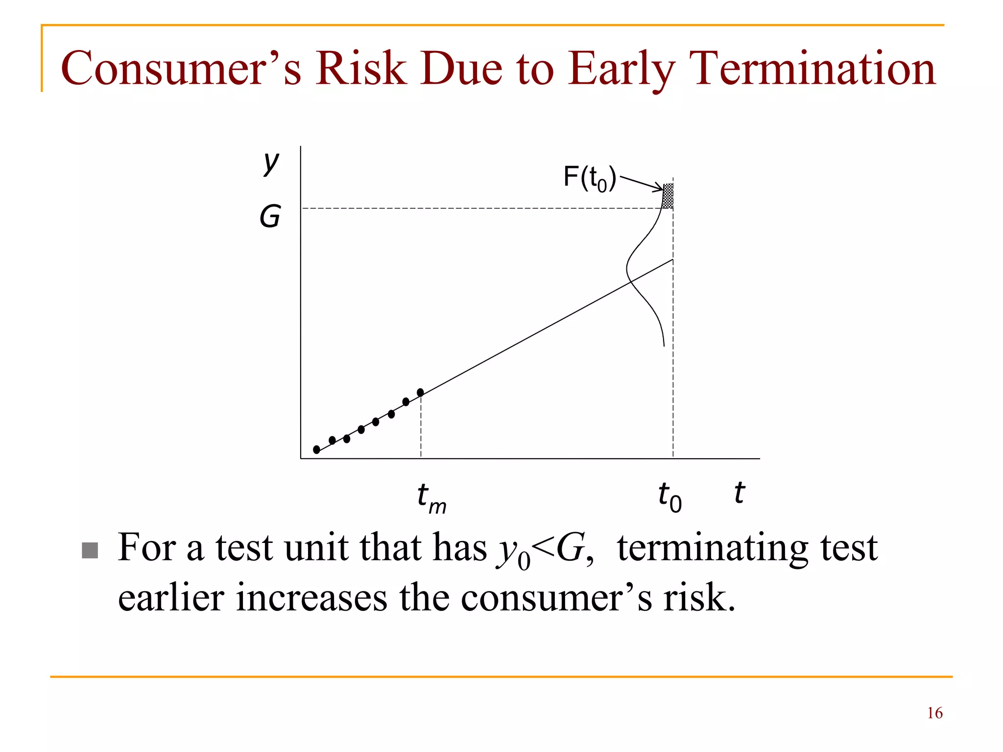
](https://image.slidesharecdn.com/efficientreliabilitydemonstrationtests-140609150614-phpapp02/75/Efficient-Reliability-Demonstration-Tests-by-Guangbin-Yang-15-2048.jpg)

This document discusses efficient reliability demonstration tests that can reduce sample sizes and test times compared to conventional methods. It presents principles for test time reduction using degradation measurements during testing. Methods are provided for calculating optimal test plans that minimize costs while meeting reliability requirements and risk constraints. Decision rules are given for terminating tests early based on degradation measurements and risk estimates. An example application demonstrates how the approach can significantly reduce testing costs.