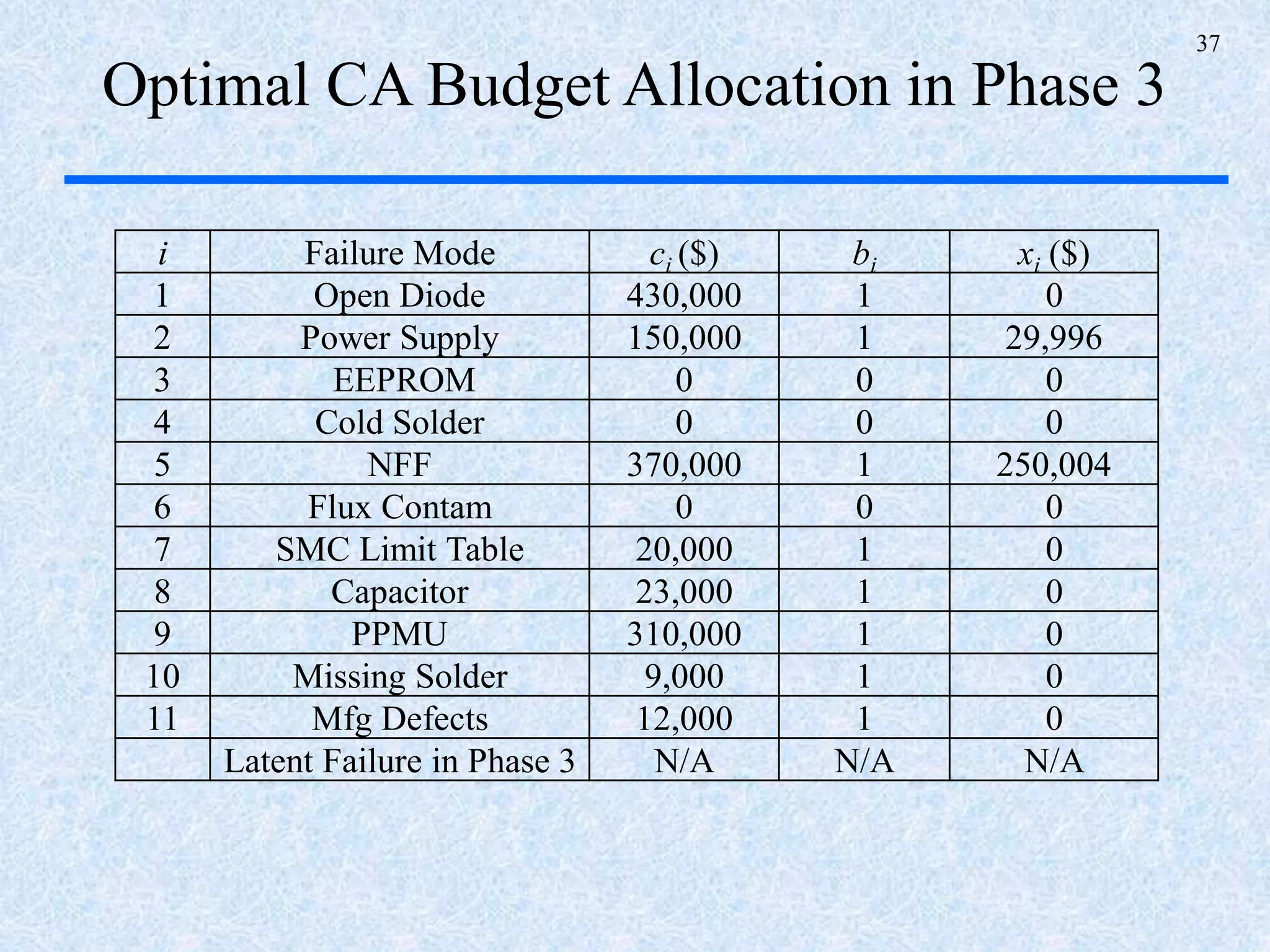
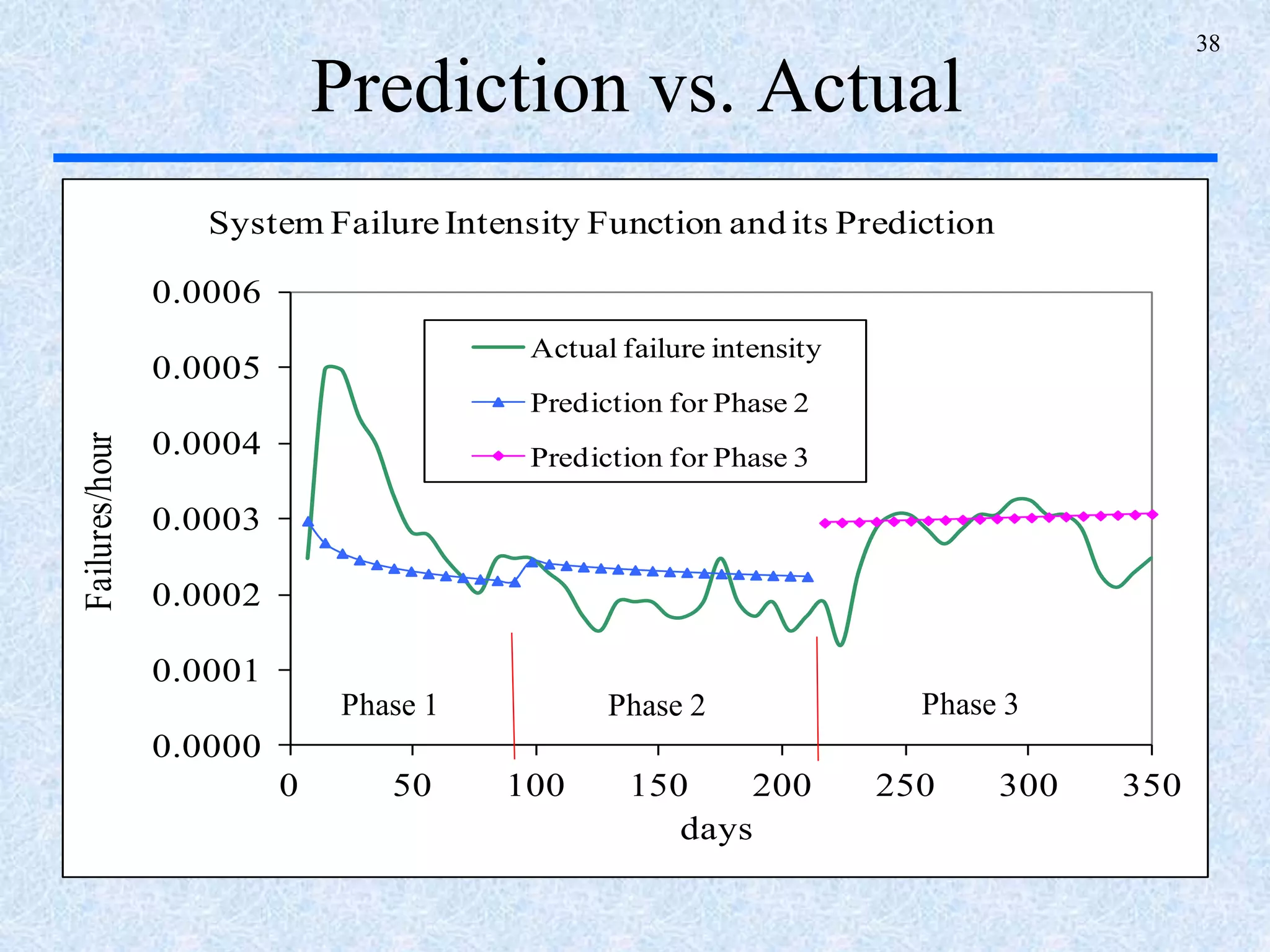
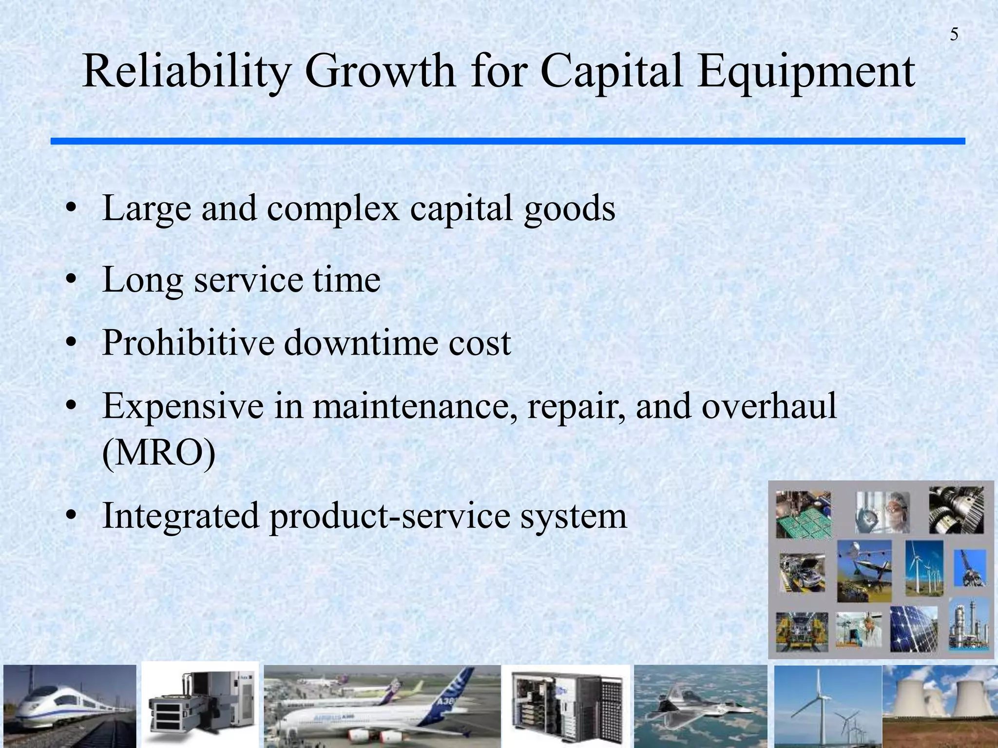
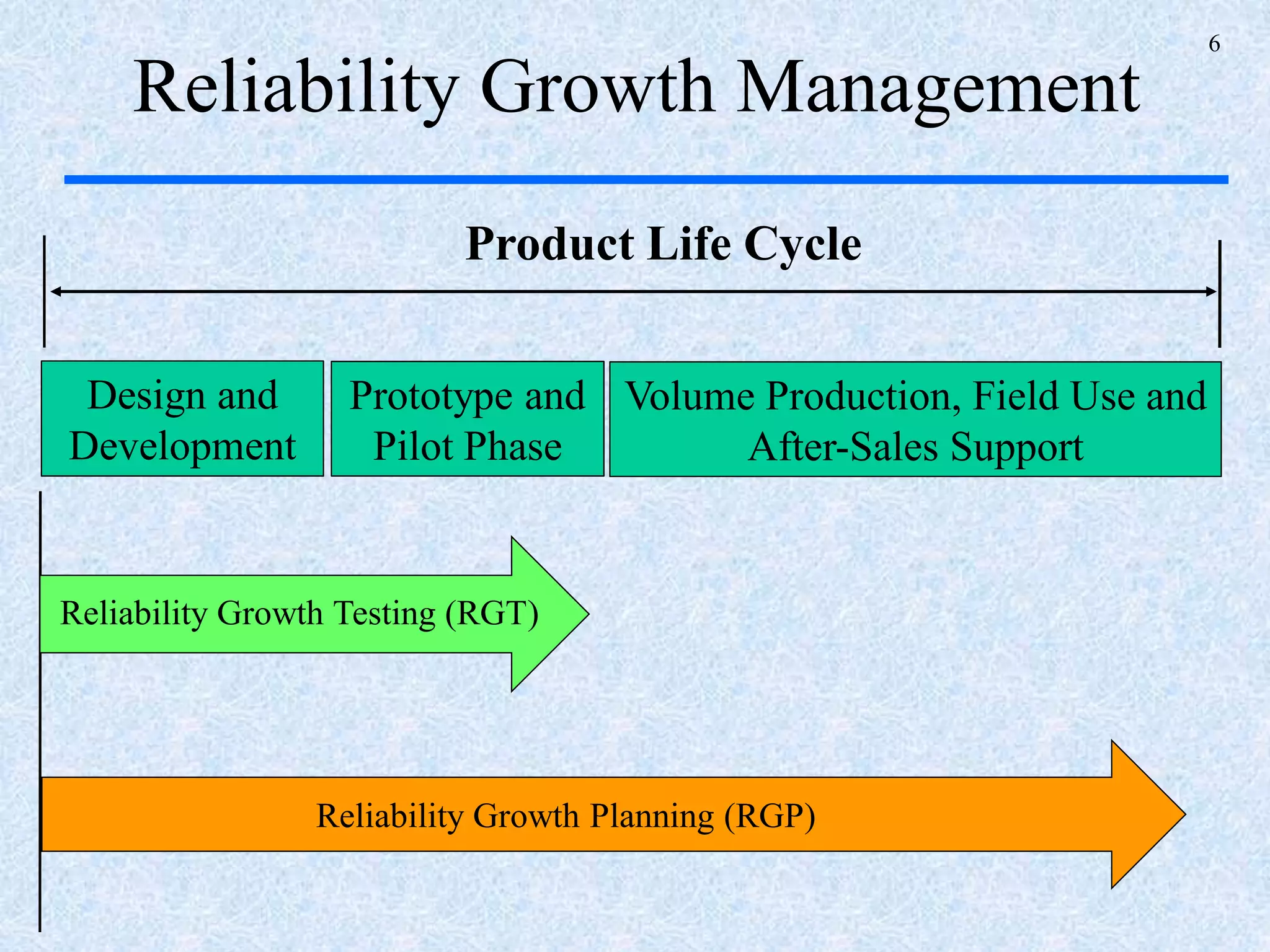
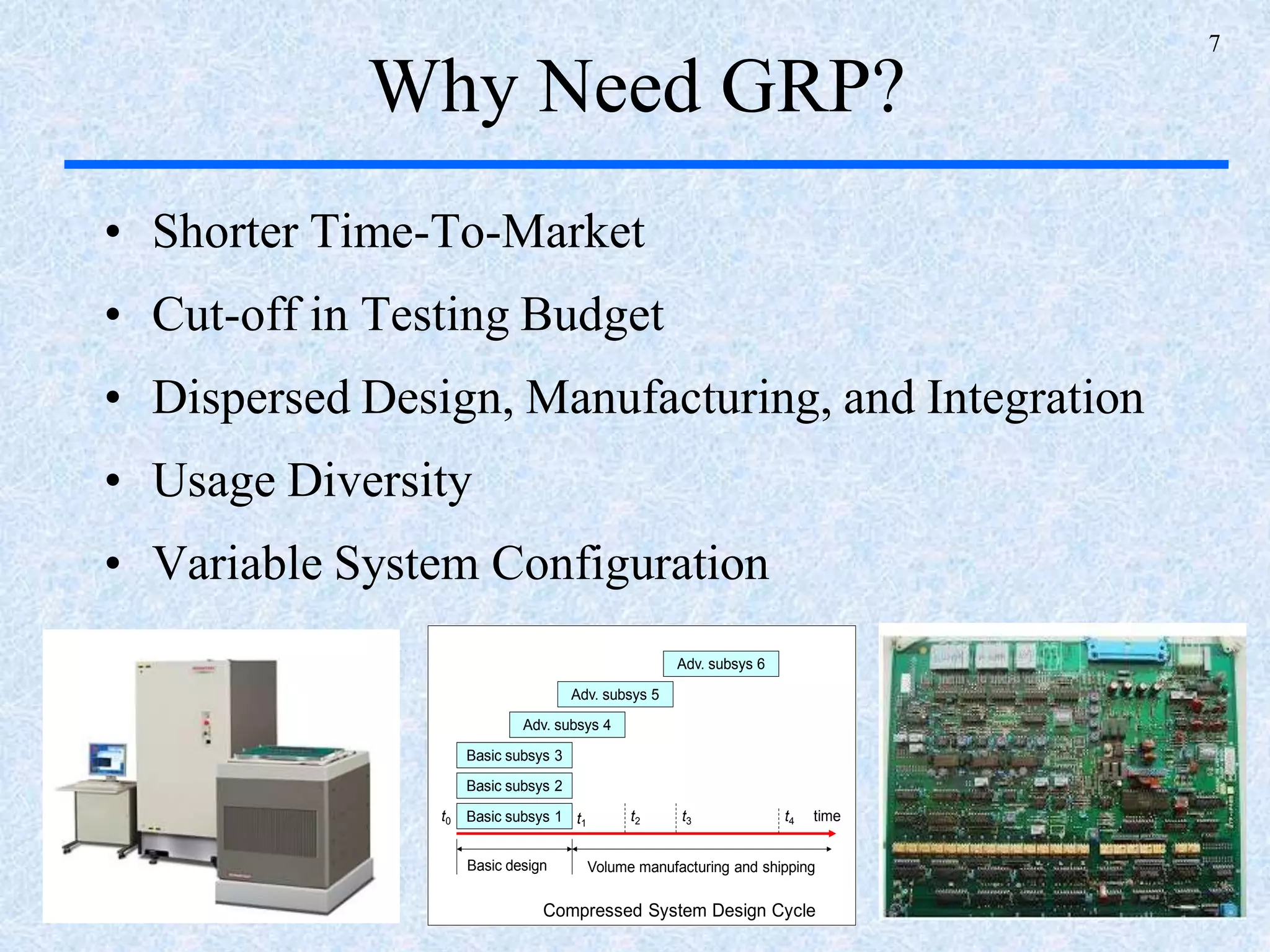
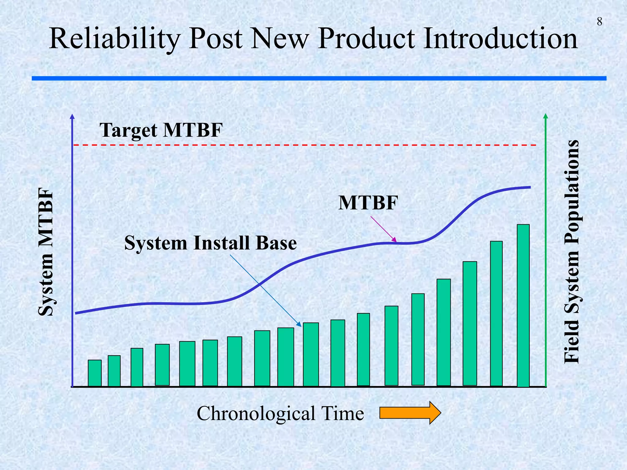
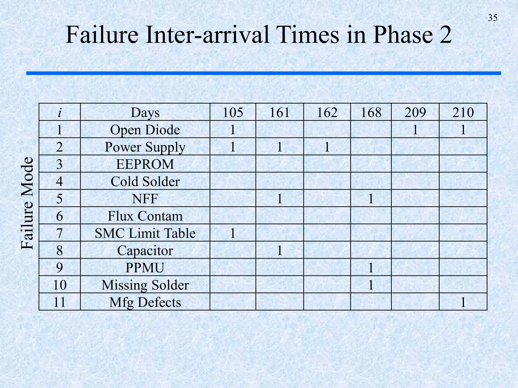
The document discusses a multi-phase approach to reliability growth planning in manufacturing, especially considering latent failure modes and their impact on electronic equipment. It outlines the need for reliability growth planning to reduce downtimes and costs while managing complex capital goods and details prediction methods for both surfaced and latent failure modes. Additionally, it presents a numerical example illustrating the allocation of resources and corrective actions to enhance reliability throughout various phases of product lifecycle.

1. A Multi-Phase Decision on
Reliability Growth with Latent
Failure Modes
(下一代制造业可靠性增长计
划的多级决策)
Tongdan Jin, Ph.D.
©2014 ASQ
http://www.asqrd.org

2. 2
A Multi-Phase Decision on Reliability Growth
with Latent Failure Modes
Tongdan Jin, Ph.D.
Ingram School of Engineering
Texas State University, TX 78666, USA
6pm Pacific Time on Feb. 9, 2014

3. 3
Contents
• The Needs for Reliability Growth Planning
• Reliability Growth considering Latent Failure Modes
• Multi-Phase Reliability Growth Management
• Applications to Electronic Equipment
• Conclusion

4. 4
Topic I:
Reliability Growth Test (RGT)
Vs.
Reliability Growth Planning (RGP)

5. 5
Reliability Growth for Capital Equipment
• Large and complex capital goods
• Long service time
• Prohibitive downtime cost
• Expensive in maintenance, repair, and overhaul
(MRO)
• Integrated product-service system

6. 6
Reliability Growth Management
Design and
Development
Prototype and
Pilot Phase
Volume Production, Field Use and
After-Sales Support
Product Life Cycle
Reliability Growth Testing (RGT)
Reliability Growth Planning (RGP)

7. 7
Why Need GRP?
• Shorter Time-To-Market
• Cut-off in Testing Budget
• Dispersed Design, Manufacturing, and Integration
• Usage Diversity
• Variable System Configuration
Basic subsys 1
Basic subsys 2
time
Basic subsys 3
Basic design Volume manufacturing and shipping
Adv. subsys 4
Adv. subsys 5
Adv. subsys 6
t1
t2 t3 t4t0
Figure 3 Compressed System Design Cycle

8. 8
Reliability Post New Product Introduction
MTBF
System Install Base
SystemMTBF
FieldSystemPopulations
Chronological Time
Target MTBF

9. 9
Different MTBF Scenarios
TimeTime (month)
Forecasted
Observed by OEM
Experienced by customer

10. 10
System Failure Mode Categories
Failures Breakdown by Root-Cause Catagory
0%
10%
20%
30%
40%
50% Hardware
Design
Mfg
Process
Software
NFF
Four different modules,
Data from >100 systems
shipped within one year.
A
B
C
D

11. 11
RGP Program: A Synergy of ECO and CA
Product Design
& Manufacturing
In-service
Systems
Spare
Inventory
Retrofit Loop
ECO Loop1. Failure mode analysis
2. Reliability growth
prediction
3. CA implementations
Spare
Batch
Repair
Center
Retrofit
Team
New System Shipping and Installation
ECO=Engineering Change Order
CA=Corrective Actions

12. 12
Topic II:
Reliability Prediction Based on
Surfaced Failure Modes

13. 13
Failure Intensity Rate w/o Latent Failures


n
i
iB
m
i
iAcs
tttt
1
,
1
,
)()()|( 
A,i(t)= failure intensity for failure mode i in A
B,i(t)= failure intensity for failure mode i in B
m = number of failure modes in A by time tc
n= number of failure modes in B by time tc
Where:
Time t0
Failureintensity
No trends
1(t)
2(t)
3(t)
4(t)
Trends
tc
a
b
c
d

14. 14
Crow/AMSAA Growth Model
 









N
i
i
s
t
t
N
1
ln
ˆ 
 ˆ
ˆ
s
t
N

1ˆ
ˆˆ 
 
 tFailure Intensity:
2
2/1,2
ˆ
2



 N
N 2
2/,2
ˆ
2


N
N
Reject H0
Where
Hypothesis Testing:
H0: β=1, HPP
H1: β1, NHPP
or
0
1
2
3
4
5
6
0 1 2 3 4 5
FailureIntensity
Time
Various FailureIntensity Models
beta 1
beta 0.5
beta 1.5
=1 for all
ts=termination time, ti=ith failure arrival time
HPP=Homogenous Poisson Process
NHPP=Non-homogenous Poisson Process

15. 15
Failure Intensity Function
 



n
i
ii
m
i
ics
i
ttt
1
1
1
)|( 

Constant Crow/AMSSA
Eq. (2)
)(2 t

16. 16
Topic III:
Reliability Prediction considering
Latent Failure Modes

17. 17
What is the Latent Failure Mode
1. Also known as dormant failure mode
2. Hibernated
3. Depending on customer usage
4. May caused by design weakness
5. Software bugs, and
6. Electro-statistic discharge (ESD)
7. Others ….

18. 18
Surfaced & Latent Failure Modes for a Product
Days 7 14 21 84 105 161 168 210 231 266 287 315 343 350
Open Diode 1 1 2 6 7 7 7 9 15 16 16 17 17 17
Power Supply 0 1 1 1 2 4 4 4 4 4 6 6 7 7
Corupt ID Prom 0 2 2 2 2 2 2 2 2 2 2 2 2 2
Cold Solder 0 0 1 1 1 1 1 1 1 1 1 1 1 1
NFF 0 0 0 1 1 2 3 3 4 6 6 6 6 6
FluxContam 0 0 0 1 1 1 1 1 1 1 1 1 1 1
SMC Limit Table 0 0 0 0 1 1 1 1 1 1 1 1 1 1
Capacitor 0 0 0 0 0 1 1 1 1 1 1 1 1 1
PPMU 0 0 0 0 0 0 1 1 1 1 1 2 2 2
missing solder 0 0 0 0 0 0 1 1 1 1 1 1 1 1
Mfg defect 0 0 0 0 0 0 0 1 1 1 1 1 1 1
Bad ASIC 0 0 0 0 0 0 0 0 1 1 1 1 1 1
Fuse 0 0 0 0 0 0 0 0 0 1 1 1 1 1
Open Trace 0 0 0 0 0 0 0 0 0 0 1 1 1 1
Op-Amp 0 0 0 0 0 0 0 0 0 0 0 2 2 2
Timing Generator 0 0 0 0 0 0 0 0 0 0 0 1 1 1
Solder Short 0 0 0 0 0 0 0 0 0 0 0 0 1 1
Total per week 1 4 6 12 15 19 22 25 33 37 40 45 47 47
Number in the cell represent the failures observed between two consecutive time window.
FailureMode

19. 19
Surfaced and Latent Failure Modes
Surfaced
Latent
Latent
A latent failure mode becomes a surfaced once it occurred.

20. 20
Reliability Model with Latent Failure Modes




k
j
j
n
i
ii
m
i
ics
tttt i
11
1
1
)()|(  
• k=the number of new latent failure modes occurred in T.
• γj(t) =the failure intensity for the jth latent failure mode.
• Where t>tc.
Where
Projected latent failure
intensity after tc.

21. 21
Estimate Cumulative Latent Failure Intensity
)()|(
1
1
1
tttt a
n
i
ii
m
i
ics
i
  








k
j
j
n
i
ii
m
i
ics
tttt i
11
1
1
)()|(  
 

ck
j
cj
c
a
k
j
j Tt
T
T
tt
11
)()()( 
(kc=# of latent failure
modes occurred in Tc)
where















c
c
c
cc
T
Tk
tt
ttk
k
0
)(
Eq. (4)
Eq. (5)
Eq. (3)

22. 22
Summary of Latent Failure Mode Prediction
• Step 1: Estimate i(t) for surfaced failure mode i at tc
using Crow/AMSAA model
• Step 2: Obtain s(t|tc) using Eq. (2) on slide 14.
• Step 3: Estimate k and Γa(t) using Eq. (4) and (5)
• Step 4: Obtain the reliability growth model Eq. (3)
For more details, please also refer to T. Jin, H. Liao, M. Kilari, “Reliability growth modeling
for in-service systems considering latent failure modes,” Microelectronics Reliability, vol. 50,
no. 3, 2010, pp. 324-331.

23. 23
Topic IV:
Reliability Growth Planning
Under
Budget/Cost Constraints

24. 24
Recourses ($)
Spent on CA due to
1. Retrofit
2. ECO
Links:
$ of CA and
% reduction of a
failure mode
CA
Effectiveness
Function
Why Need the CA Effectiveness Estimate

25. 25
0 c
x
1
effectiveness
b
c
x
xh 





)(
h(x)
CA budget ($)
Effectiveness Model
b>1
b=1
b<1
Modeling CA (or Fix) Effectiveness
b and c to be determined
Effectiveness=
Failure rate before CA – Failures rate after CA
Failure rate before CA
For more details on effectiveness function, please refer to T. Jin, Y. Yu, and F. Belkhouche, “Reliability growth using retrofit or
engineering change order-a budget-based decision making,” in Proceedings of IERC Conference, 2009, pp. 2152-2157.

26. 26
An Example: ECO or Retrofit
A type of relays used on a PCB module fails constantly due to
a known failure mechanism. Two options available for
corrective actions
1. Replace all on-board relays upon the failure return of the
module
2. Pro-actively recall all modules and replace with new types
of relays having much higher reliability
CA Option Cost ($) CA Effectiveness
ECO Low Low
Retrofit High High

27. 27
An Illustrative Example
The current failure rate a type of relay is 210-8 faults per
hour. Upon the implementation of CA, the rate is reduced to
510-9.
The CA effectiveness can be expressed as 0.75, that is
75.0
102
105102
8
98






28. 28
Incorporate h(x) into
b
c
x
xh 





)(
)|( cs tt
)(11);(
11
11
tt
c
x
c
x
t a
c
x
ii
n
i
b
i
i
m
i
i
b
i
i
s
i
ib
i
i
ii























































 x
)()|(
1
1
1
tttt a
n
i
ii
m
i
ics
i
  





29. 29
Optimization Formulation
Min:
Subject to:
xi0 for i=1, 2, …., m
Where
,
}


m
i
ixg
1
)(x
0);(  ts x
xi=CA budget for failure mode i, for i=1, 2, …, m.
0= target system failure intensity
RGP budget
Target reliability

30. 30
Topic V:
Numerical Example
(Driving Electronic Equipment
Reliability)
The example is taken from the following paper:
T. Jin, Y. Yu, H.-Z. Huang, “A multiphase decision model for reliability growth considering
stochastic latent failures,” IEEE Transactions on Systems, Man and Cybernetics, Part A,
vol. 43. no. 4, 2013, pp. 958-966.

31. 31
Overview of The Planning Horizon
Phase 1
Day 1-90
Phase 2
Day 91-220
Phase 3
Day 221-350
• Collect field data
• Identify surface failure
modes
• Reliability prediction for
Phase 2
• Resource allocation for
Phase 2
• Collect field data
• Identify latent failure
modes
• Reliability prediction
• Implement CA/ECO
• Resource allocation for
Phase 3
• Collect field data
• Identify new latent failure
modes
• Reliability prediction
• Implement CA/ECO
• Resource allocation for
Phase 4 (next)

32. 32
Failure Inter-Arrival Times in Phase 1
i Days 7 14 15 21 84 85 87 89
1 Open Diode 1 1 1 1 1 1
2 Power Supply 1
3 EEPROM 1 1
4 Cold Solder 1
5 NFF 1
6 Flux Contam 1
FailureMode
Note: Numbers in the cell represents the failure quantity.

33. 33
i Failure Mode
1 Open Diode 1.29E-6 1.413 2.28E-4 5.2174E-10
2 Power Supply 1.91E-5 1.00 1.91E-5 3.6398E-12
3 EEPROM 5.40E-3 0.544 1.42E-5 2.0126E-12
4 Cold Solder 1.91E-5 1.00 1.91E-5 3.6398E-12
5 NFF 1.91E-5 1.00 1.91E-5 3.6398E-12
6 Flux Contam 1.91E-5 1.00 1.91E-5 3.6398E-12
7 Latent Failures 2.39E-4 1.021 3.07E-4 9.4433E-10
iˆ
iˆ )](ˆ[ tE i ))(ˆvar( ti
Reliability Forecasting for Phase 2FailureMode

34. 34
Optimal CAAllocation in Phase 2
i Failure Mode ci ($) bi xi ($)
1 Open Diode 430,000 1 412,790
2 Power Supply 150,000 1 0
3 EEPROM 250,000 1 0
4 Cold Solder 75,000 1 19,510
5 NFF 370,000 1 0
6 Flux Contamination 45,000 1 27,700
7 Latent Failures (Phase 2)
N/A N/A N/A
N/A=not applicable
FailureMode

35. 35
Failure Inter-arrival Times in Phase 2
i Days 105 161 162 168 209 210
1 Open Diode 1 1 1
2 Power Supply 1 1 1
3 EEPROM
4 Cold Solder
5 NFF 1 1
6 Flux Contam
7 SMC Limit Table 1
8 Capacitor 1
9 PPMU 1
10 Missing Solder 1
11 Mfg Defects 1
FailureMode

36. 36
i Failure Mode
1 Open Diode 2.30E-4 0.903 6.40E-5 4.09E-11
2 Power Supply 2.66E-5 1.02 3.40E-5 1.16E-11
3 EEPROM 2.51E-2 0.374 4.49E-6 2.02E-13
4 Cold Solder 8.27E-6 1.00 8.27E-6 6.83E-13
5 NFF 4.22E-11 2.14 9.46E-5 8.94E-11
6 Flux Contam 8.27E-6 1.00 8.27E-6 6.83E-13
7 SMC Limit Table 8.27E-6 1.00 8.27E-6 6.83E-13
8 Capacitor 8.27E-6 1.00 8.27E-6 6.83E-13
9 PPMU 8.27E-6 1.00 8.27E-6 6.83E-13
10 Missing Solder 8.27E-6 1.00 8.27E-6 6.83E-13
11 Mfg Defects 8.27E-6 1.00 8.27E-6 6.83E-13
Latent Failure in
Phase 3 8.46E-6 1.208 1.07E-4 1.15E-10
iˆ
iˆ )](ˆ[ tE i ))(ˆvar( ti
Reliability Forecasting for Phase 2

37. 37
Optimal CA Budget Allocation in Phase 3
i Failure Mode ci ($) bi xi ($)
1 Open Diode 430,000 1 0
2 Power Supply 150,000 1 29,996
3 EEPROM 0 0 0
4 Cold Solder 0 0 0
5 NFF 370,000 1 250,004
6 Flux Contam 0 0 0
7 SMC Limit Table 20,000 1 0
8 Capacitor 23,000 1 0
9 PPMU 310,000 1 0
10 Missing Solder 9,000 1 0
11 Mfg Defects 12,000 1 0
Latent Failure in Phase 3 N/A N/A N/A

38. 38
Prediction vs. Actual
0.0000
0.0001
0.0002
0.0003
0.0004
0.0005
0.0006
0 50 100 150 200 250 300 350
Failures/hour
days
System Failure Intensity Function and its Prediction
Actual failure intensity
Prediction for Phase 2
Prediction for Phase 3
Phase 1 Phase 2 Phase 3

39. 39
Conclusions
1. New designs are often subject to both components (hardware)
and non-components failures. Some failure modes are dormant.
2. RGP is a multi-disciplinary cross-function team effort as it
involves design, manufacturing, testing, operation,
maintenance as well as latent failures.
3. We proposes a CA effectiveness function and further integrates
it into the RGP model to achieve reliability target a lower cost.
4. An accurate reliability growth prediction is useful, yet it is
more beneficial to industry as when to reach the reliability goal
and how much resource (labor and budget) is required.

40. 40
References
1. D. S. Jackson, H. Pant, M. Tortorella, “Improved reliability-prediction and field-reliability-data analysis for field-
replaceable units,” IEEE Transactions on Reliability, vol. 51, no. 1, 2002, pp. 8-16.
2. J. T. Duane, “Learning curve approach to reliability monitoring,” IEEE Transactions on Aerospace, vol. 2, no. 2, 1964, pp.
563-566.
3. L. H. Crow, “Reliability analysis for complex, repairable systems,” SIAM Reliability and Biometry, 1974, pp. 379-410.
4. M. Xie, M. Zhao, “Reliability growth plot-an underutilized tool in reliability analysis,” Microelectronics and Reliability,
vol. 36, no. 6, 1996, pp. 797-805.
5. D. W. Coit, “Economic allocation of test times for subsystem-level reliability growth testing,” IIE Transactions on Quality
and Reliability Engineering, vol. 30, no. 12, 1998, pp. 1143-1151.
6. M. Krasich, J. Quigley, L. Walls, “Modeling reliability growth in the system design process,” in Proceedings of Annual
Reliability and Maintainability Symposium, 2004, pp. 424-430.
7. S. Inoue, S. Yamada, “Generalized discrete software reliability modeling with effect of program size,” IEEE Transactions on
Systems, Man and Cybernetics, Part A, vol. 37, no. 2, 2007, pp. 170-179.
8. P. M. Ellner, J. B. Hall, “An approach to reliability growth planning based on failure mode discovery and correction using
AMSAA projection methodology,” in Proceedings of Annual Reliability and Maintainability Symposium, 2006, pp. 266-
272.
9. T. Jin, H. Liao, M. Kilari, “Reliability growth modeling for in-service systems considering latent failure modes,”
Microelectronics Reliability, vol. 50, no. 3, 2010, pp. 324-331.
10. T. Jin, Y. Yu, H.-Z. Huang, "A multiphase decision model for reliability growth considering stochastic latent failures," IEEE
Transactions on Systems, Man and Cybernetics, Part A, vol. 43. no. 4, 2013, pp. 958-966.
11. L. Attardi, G. Pulcini, “A new model for repairable systems with bounded failure intensity,” IEEE Transactions on
Reliability, vol. 54, no. 4, 2005, pp. 572-582.
12. M. S. Bazaraa, C. M. Shetty, Nonlinear Programming: Theories and Applications, 3rd edition, 2006, John Wiley & Sons,
New York.

41. 41
Thank you
And
Questions ?
Email: tj17@txstate.edu