This document discusses using degradation data to model reliability and predict failure times. It begins by explaining how failures can be caused by degradation over time in mechanical components and integrated circuits. Examples of degradation mechanisms like creep, fatigue, and corrosion are provided. The document then discusses using non-destructive and destructive inspection of degradation parameters to build models and predict reliability. Accelerated degradation testing is also covered as a way to quickly generate degradation data under elevated stress conditions. Overall, the document provides an overview of modeling reliability using degradation data and predicting failure times based on degradation paths.

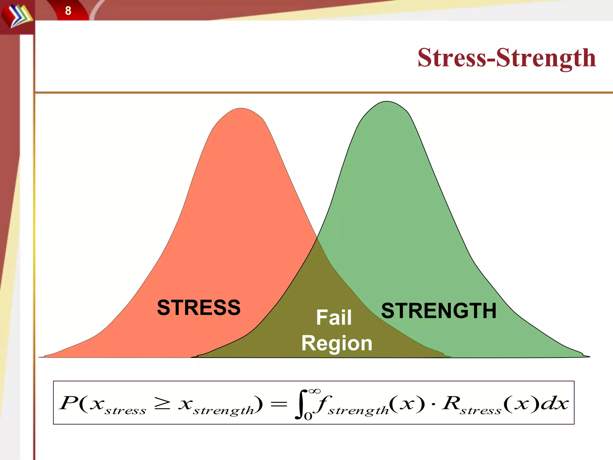
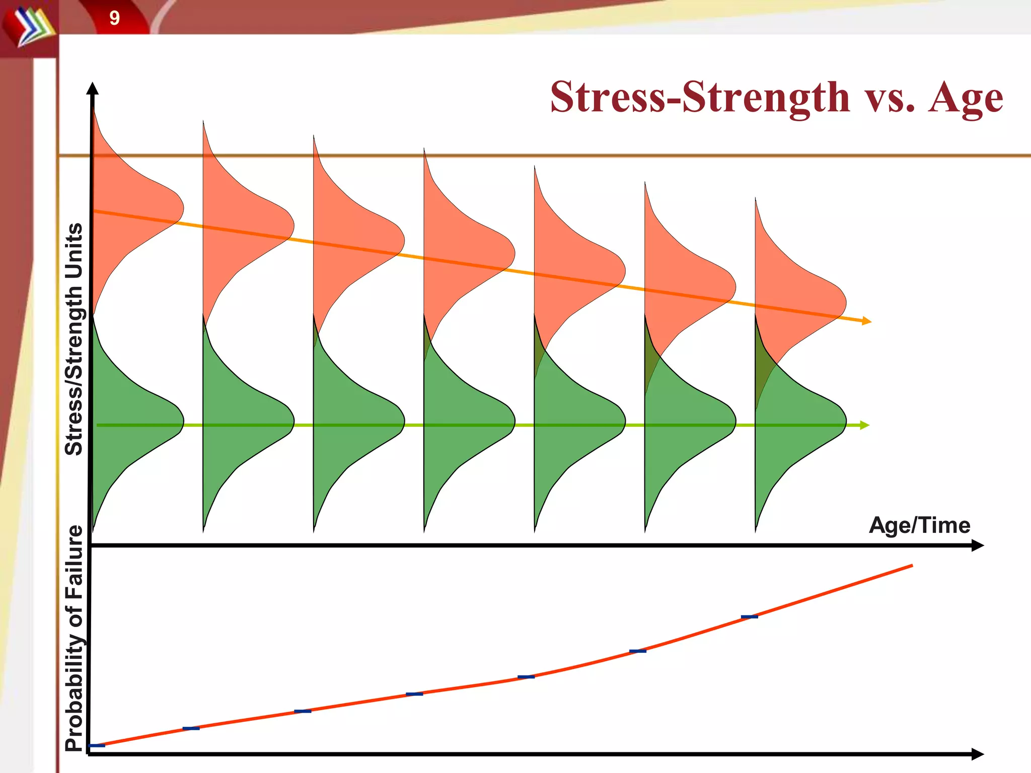
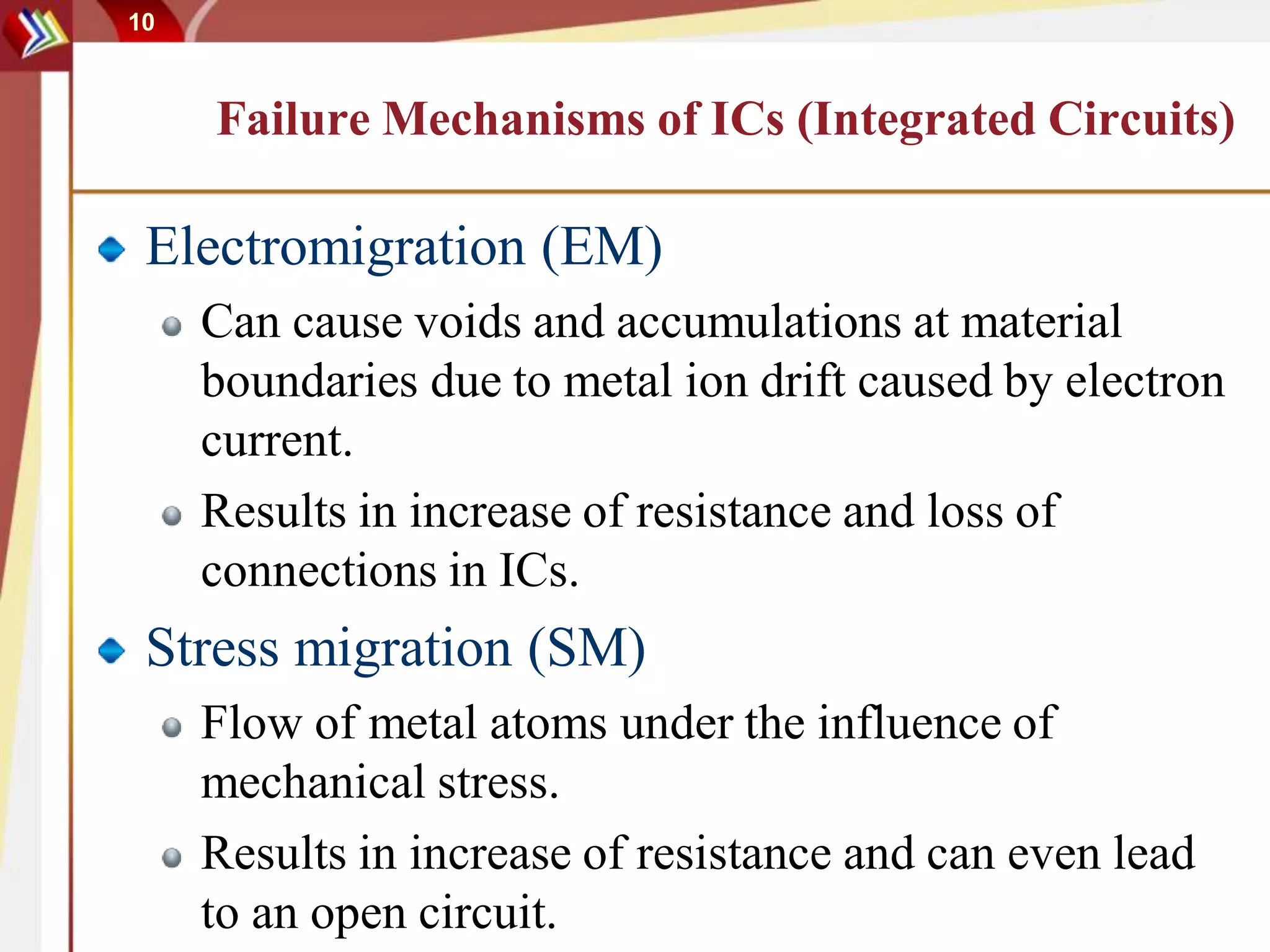
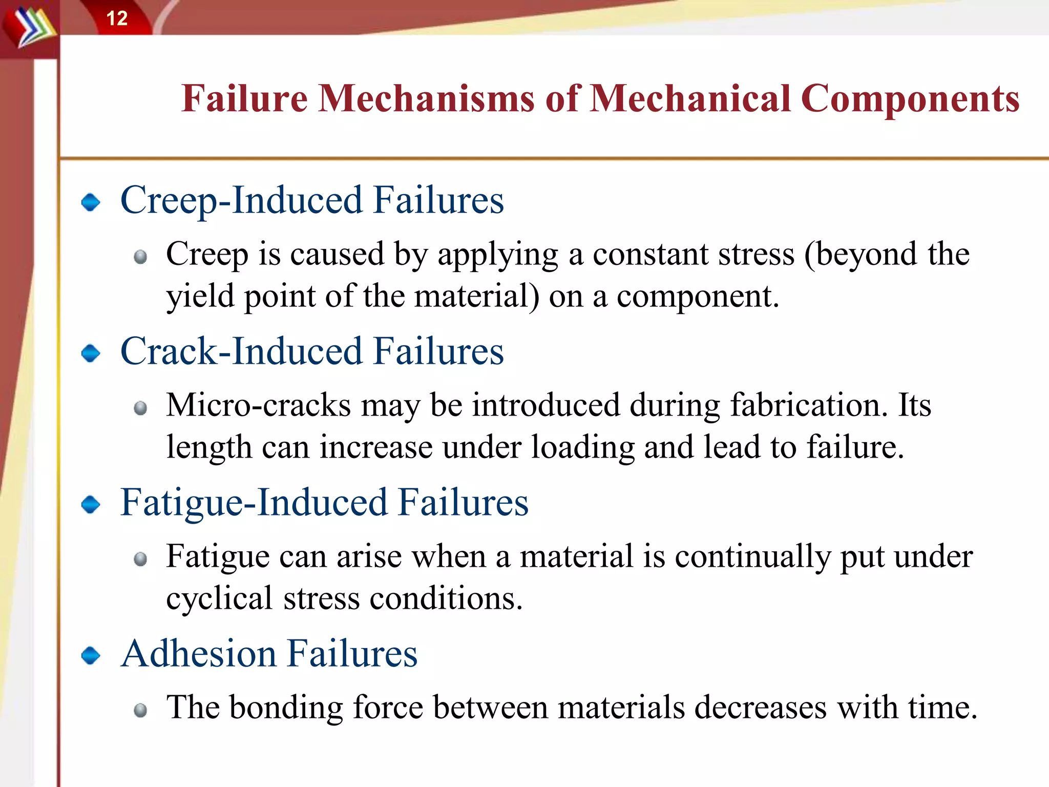
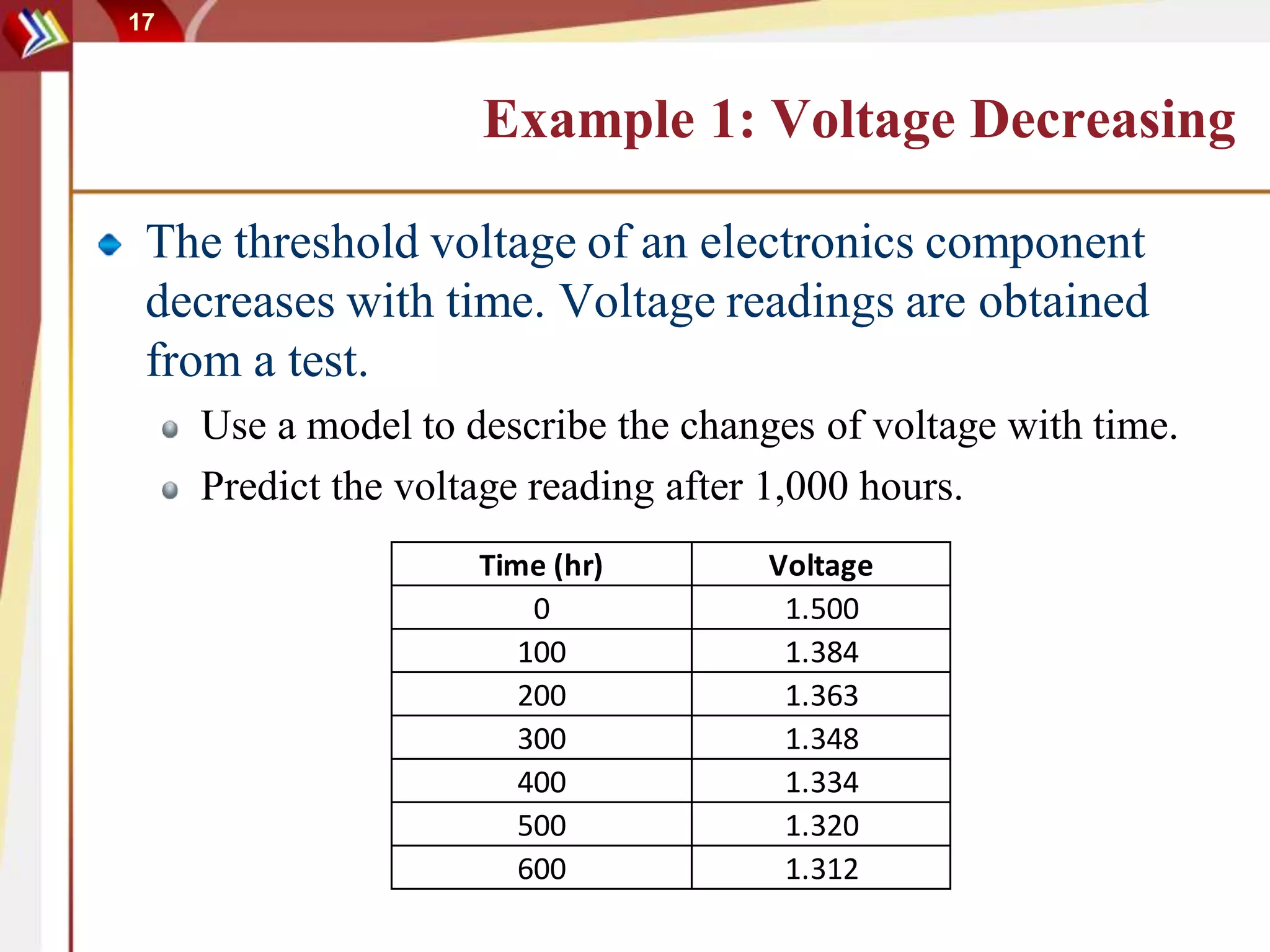
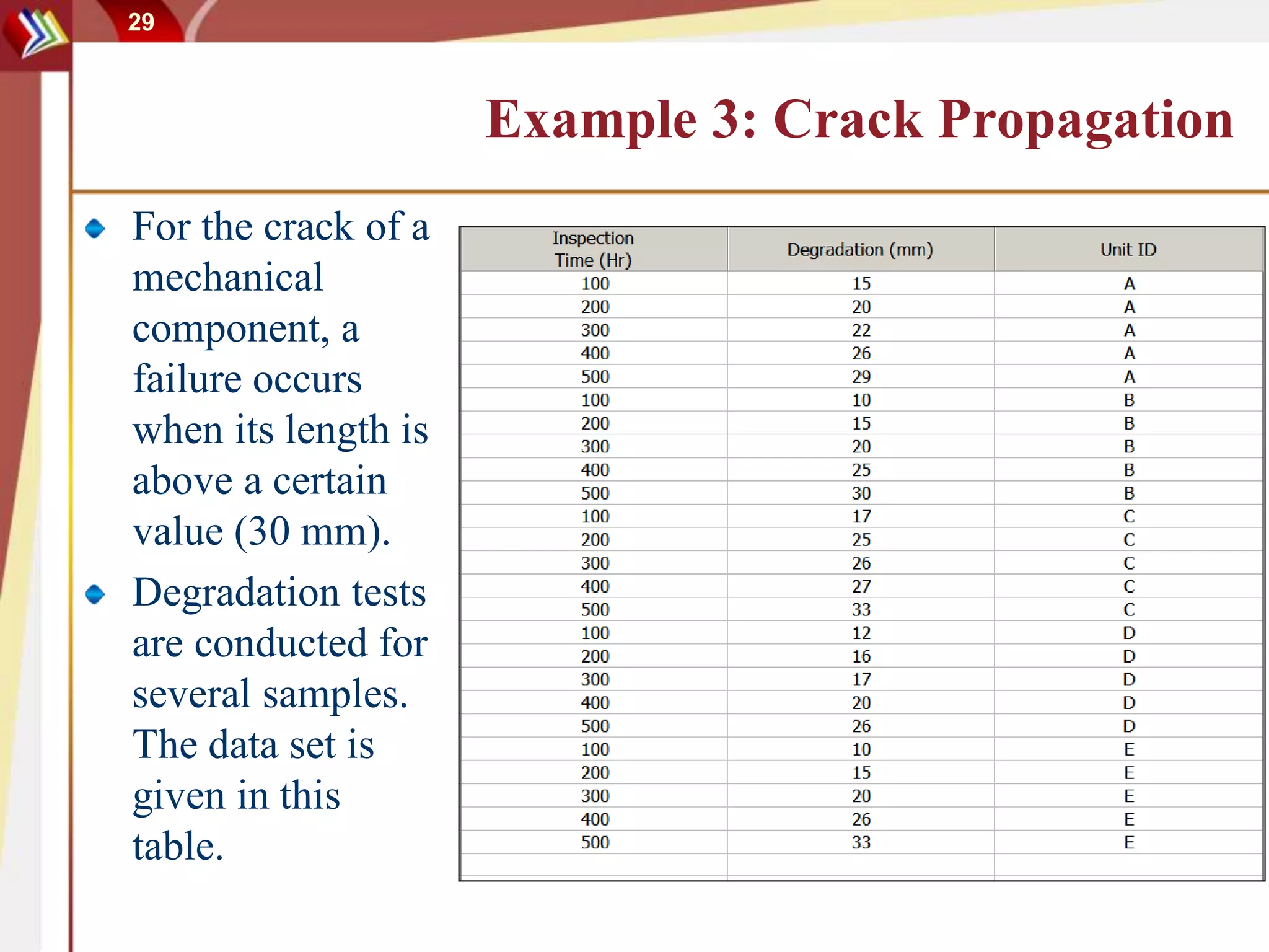
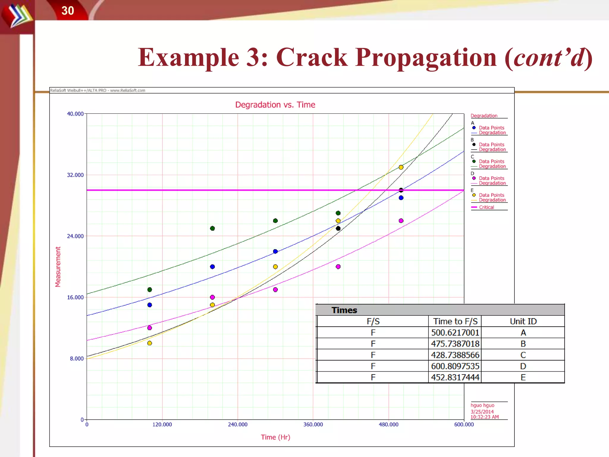
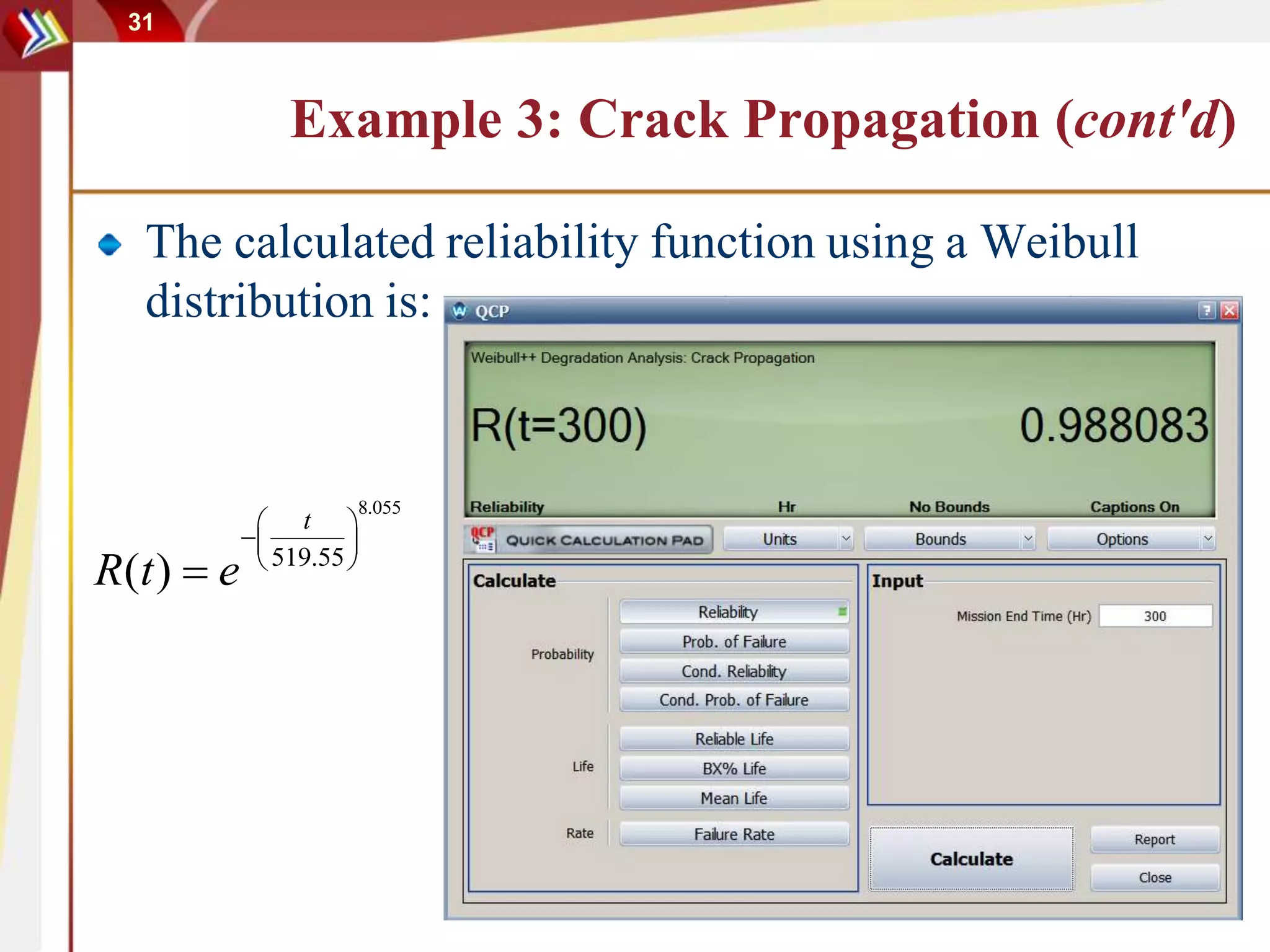
1. Reliability Modeling Using
Degradation Data
利用退化数据进行可靠性
预计
Harry Guo

2. ASQ Reliability Division
Chinese Webinar Series
One of the monthly webinars
on topics of interest to
reliability engineers
To view upcoming or recorded webinars visit us today at
www.asqrd.org

3. ©1992-2014 ReliaSoft Corporation - ALL RIGHTS RESERVED
利用退化数据进行可靠性预计
(Reliability Modeling Using Degradation Data)
郭怀瑞 (Harry Guo)
Ph.D., CRE, CQE, CRP

4. 4
Outlines
Part 1: Failures caused by degradation
Examples of integrated circuits (ICs)
Examples of mechanical components
Part 2: Using degradation data to predict
component reliability
Non-destructive inspection
Destructive inspection
Part 3: Accelerated degradation data analysis

5. 5
EDUCATION
5
Part I: Failures Caused by Degradation

6. 6
Why Failure Occurs
Failures can occur for many different reasons.
Design incapability
Being overstressed
Manufacturing defects
Wearout
User error
…

7. 7
Wearout Failure
Failures can be caused by component properties
changing over time.
Adequate initial quality doesn’t ensure high reliability.
Component performance can decrease very quickly.
Material strength decreases over time.
Corrosion, insulation and voltage deteriorate with time.
A failure occurs, when degradation reaches a critical value.
Wearout failures are time dependent.
Failure rate increases with time.

8. 8
Stress-Strength
STRESS STRENGTHFail
Region
dxxRxfxxP stressstrengthstrengthstress )()()(
0
 


9. 9
Stress-Strength vs. Age
Age/Time
Stress/StrengthUnitsProbabilityofFailure

10. 10
Failure Mechanisms of ICs (Integrated Circuits)
Electromigration (EM)
Can cause voids and accumulations at material
boundaries due to metal ion drift caused by electron
current.
Results in increase of resistance and loss of
connections in ICs.
Stress migration (SM)
Flow of metal atoms under the influence of
mechanical stress.
Results in increase of resistance and can even lead
to an open circuit.

11. 11
Failure Mechanisms of ICs (cont'd)
Corrosion
Corrosion tests are usually conducted under high
temperature and high humidity.
Corrosion activity is measured by monitoring the resistance
versus time.
Time-Dependent Dielectric Breakdown (TDDB)
Caused by dielectric degradation in electric fields.
Current density increases dramatically and voltage drops to
0 when TDDB occurs.
This is a destructive test. The component is destroyed after
TDDB occurs.

12. 12
Failure Mechanisms of Mechanical Components
Creep-Induced Failures
Creep is caused by applying a constant stress (beyond the
yield point of the material) on a component.
Crack-Induced Failures
Micro-cracks may be introduced during fabrication. Its
length can increase under loading and lead to failure.
Fatigue-Induced Failures
Fatigue can arise when a material is continually put under
cyclical stress conditions.
Adhesion Failures
The bonding force between materials decreases with time.

13. 13
EDUCATION
13
Part II: Using Degradation Data
to Predict Reliability

14. 14
Degradation Analysis: Non-Destructive
This type of analysis involves the
measurement of degradation or
performance over time.
Degradation data is also called parameter
data. Use a parameter or index to indicate
the status of a component.
The degradation path/curve can be
described by a mathematical function.
Failure can be directly related to the
amount of degradation.

15. 15
Degradation Data – Crack Length Example
An example of degradation data
involves the length of cracks in
turbine blades. A failure is
defined as a crack length of 1.6
inches or greater. A specimen is
tested to 120,000 cycles, at
which point the crack length is
1.27 inches.
Even though the crack in the
test specimen did not reach the
critical length, it is a simple
matter to extrapolate the test
data to the point at which the
degradation would reach the
critical level (177,480 cycles).
0.8
0.9
1
1.1
1.2
1.3
1.4
1.5
1.6
1.7
1.8
0 50000 100000 150000 200000
Cycles
Cracklength(inches)
0.8
0.9
1
1.1
1.2
1.3
1.4
1.5
1.6
1.7
1.8
0 50000 100000 150000 200000
Cycles
Cracklength(inches)
177480

16. 16
Mathematical Models for Degradation Path
The commonly used degradation models are the
following simple models:
Linear: 𝒚 = 𝒂 ∙ 𝒕 + 𝒃
Exponential: 𝒚 = 𝒃 ∙ 𝒆 𝒂∙𝒕
Power: 𝒚 = 𝒃 ∙ 𝒕 𝒂
Logarithmic: 𝒚 = 𝒂 ∙ 𝒍𝒏 𝒕 + 𝒃
where
• 𝑦 represents the degradation performance or the percentage of
change from the initial value,
• 𝑡 represents time, and 𝑎 and 𝑏 are model parameters to be
solved for.

17. 17
Example 1: Voltage Decreasing
The threshold voltage of an electronics component
decreases with time. Voltage readings are obtained
from a test.
Use a model to describe the changes of voltage with time.
Predict the voltage reading after 1,000 hours.
Time (hr) Voltage
0 1.500
100 1.384
200 1.363
300 1.348
400 1.334
500 1.320
600 1.312

18. 18
Solution for Example 1
The following power model is used
𝑉𝑡 = 𝑉0(1 − 𝑏 × 𝑡 𝑎
)
This function can be converted to a simple linear
regression function:
𝑌 = 𝑏′ + 𝑎 × 𝑙𝑛(𝑡)
where: 𝑌 = ln( 𝑉0−𝑉 𝑡
𝑉0
) , 𝑏′
= ln 𝑏 .
The final function is:
𝑉𝑡 = 1.5 (1 − 0.021 × 𝑡 0.278
)

19. 19
Solution for Example 1 (cont'd)
The predicted voltage at 1,000 hours is:
1.5 1 − 0.021 × 1,000 0.278
= 1.284

20. 20
Degradation with Multiple Stages
Sometimes the degradation path is an S-shaped
curve.
This is for cases when degradation has multiple
stages.
Degradation behaviors are different at different
stages.
We can use either piecewise regression or an S-
shaped curve to describe the degradation.

21. 21
Example 2: Pressure Drop of a Material
A material is used in surgery to hold a certain
pressure to prevent body fluid leakage. The
pressure will decrease after the material is
deployed.
The material should meet the pressure requirement
after a certain time of use.
The engineering team wants to study how the
pressure degrades and then make design changes to
adjust the initial pressure value.

22. 22
Example 2: Pressure Drop of a Material
(cont'd)
Initial tests showed that the material
degradation experienced different stages.
Pressure quickly drops immediately after deployed.
Drop rate then slows down.
Commonly used degradation functions such as
linear, power and logarithmic do not work well
in this case.

23. 23
Example 2: Pressure Drop of a Material
(cont'd)

24. 24
Example 2: Pressure Drop of a Material
(cont'd)
It was found that modeling the percentage of pressure
drop is better than modeling the pressure directly.
This can reduce the effect of the initial value of each test
sample to the modeling.
Percentage is a value between 0 and 1, so the function
we are going to use should meet this constraint.
The function should also account for the quick change
at the beginning and slow change at the later stages.

25. 25
Example 2: Pressure of a Material (cont'd)
• A Mixed Weibull distribution is used.
• The curve can fit the observations very well.
• Based on the pressure requirement at time t, we can
calculate what the initial pressure of the material
should be.

26. 26
From Degradation to Failure Time
When degradation reaches a certain level, the
component cannot function as designed. For
example:
If the bonding force is too small, then bonded
materials will be separated.
If the voltage dropped to a critical value, then a
signal of 1 becomes a signal of 0.
The wearout of a seal will cause gas or oil leakage.
Crack length on turbine blades is too big which will
cause vibration and break the blade.

27. 27
From Degradation to Failure Time
 For each test unit, we can use a function to describe the degradation path.
 Using this function, we can predict the time when degradation will reach a
critical value.

28. 28
Reliability Prediction Using Failure Times
Once we have “failure times,” we can use them
to predict reliability.
These failure times are “predicted” pseudo failure
times from the degradation function.
This is for cases when a quantitative parameter can
be used to indicate the performance of a component.

29. 29
Example 3: Crack Propagation
For the crack of a
mechanical
component, a
failure occurs
when its length is
above a certain
value (30 mm).
Degradation tests
are conducted for
several samples.
The data set is
given in this
table.

30. 30
Example 3: Crack Propagation (cont’d)

31. 31
Example 3: Crack Propagation (cont'd)
The calculated reliability function using a Weibull
distribution is:
8.055
519.55
( )
t
R t e
 
 
 


32. 32
Degradation with Destructive Inspection
For some degradation processes, we cannot get
the degradation reading without destroying the
test samples (e.g., the breakdown voltage of
semiconductor components).
Each test sample has only one degradation
reading. Therefore, we cannot build a
degradation path for each individual test sample
as we discussed before.

33. 33
Example 4: Dielectric Breakdown Voltage
The dielectric breakdown strength of insulation
specimens decreases with time.
Each test sample was held for a certain time period at a
constant temperature, and then its breakdown voltage was
measured (a destructive test).
The insulation fails when the breakdown voltage degrades
below the design voltage 1.0 kV.
We need to estimate the reliability of the insulation
specimen based on the destructive test data.

34. 34
Example 4: Dielectric Breakdown Voltage
(cont'd)
Sample
ID
Week
Breakdown
Voltage
(KV)
Sample
ID
Week
Breakdown
Voltage
(KV)
1 1 14 17 16 6
2 1 13 18 16 6
3 1 14 19 16 5
4 1 11.5 20 16 5.5
5 2 13 21 32 2.7
6 2 11.5 22 32 2.7
7 2 13 23 32 2.5
8 2 12.5 24 32 2.4
9 4 10 25 48 1.2
10 4 11.5 26 48 1.5
11 4 11 27 48 1
12 4 9.5 28 48 1.5
13 8 6.5 29 64 1.5
14 8 5.5 30 64 1
15 8 6 31 64 1.2
16 8 6 32 64 1.2

35. 35
Example 4: Dielectric Breakdown Voltage
(cont'd)
At a given time, the
degradation value is
assumed to be a random
variable following a
distribution.
The location parameter of
the distribution is a
function of time.
The probability of getting
a degradation value
beyond the critical value
at time t is the
unreliability at time t.
( ) Pr( ( ) )critF t x t D 

36. 36
Example 4: Dielectric Breakdown Voltage
(cont'd)
We assume the degradation follows a Weibull
distribution.
The scale parameter eta (𝜂) is a function of time:
The probability of failure at time
t is:
1
( ) n
t
K t
 

 
( )
( ) Pr( ( ) ) 1
1
crit
n
crit
D
t
crit
D K t
F t x t D e
e



 
 
 
  
   
 
For example, when t = 100, the probability of failure F(100) is 0.2454.

37. 37
EDUCATION
37
Part III: Accelerated Degradation
Data Analysis

38. 38
Accelerated Degradation Test
It may take too long to test a component at the
normal use condition.
The degradation rate may be higher at elevated
stress conditions.
By testing components at higher stresses, we
can get degradation data more quickly and use
the data for reliability prediction.

39. 39
Accelerated Degradation Data Analysis
The method used to analyze accelerated degradation
data is the same as the method used for degradation data
obtained at the normal stress condition.
The degradation value is not only affected by time, it is
also affected by the stress level. The stress level affects
degradation rate.

40. 40
Non-Destructive Accelerated Degradation
Data Analysis
High
Temperature
Low
Temperature

41. 41
Example 5: Accelerated Degradation –
Non-Destructive
Consider a chemical solution (e.g., ink formulation, medicine, etc.)
that degrades with time. A quantitative measure of the quality of the
product can be obtained. This measure (QM) is said to be around 100
when the product is first manufactured and decreases with age. Any
QM higer than 50 is acceptable. Products with QM equal to or lower
than 50 are considered to be out of compliance or failed.
Engineering analysis has indicated that at higher temperatures the
QM has a higher rate of decrease. Assuming that the product’s normal
use temperature is 20oC (or 293K), the goal is to determine the shelf
life of the product via an accelerated degradation test.
“Shelf life” is defined as the time by which 10% of the products will
have a QM that is out of compliance.

42. 42
Example 5: Accelerated Degradation –
Non-Destructive (cont'd)
For this experiment, 15 samples of the product were tested, with 5
samples in each of three accelerated stress environments: 323K, 373K
and 383K. Once a month, for a period of seven months, the QM for
each sample was measured and recorded.

43. 43
Example 5: Accelerated Degradation –
Non-Destructive (cont'd)

44. 44
Degradation Results
Data for all samples were entered and individually fitted to multiple exponential
curves. From each respective curve, a time-to-failure (i.e., the time the product is
expected to go out of compliance) was automatically extrapolated.

45. 45
B10 Life Line
B10 Life

46. 46
Where to Get More Information
1. http://www.itl.nist.gov/div898/handbook/
2. www.weibull.com
3. http://www.ReliaWiki.org/index.php/ReliaSoft_Books