

![V. Krivtsov: Field Data Analysis & Statistical Warranty Forecasting | 2013 © Ford Motor Co. 12
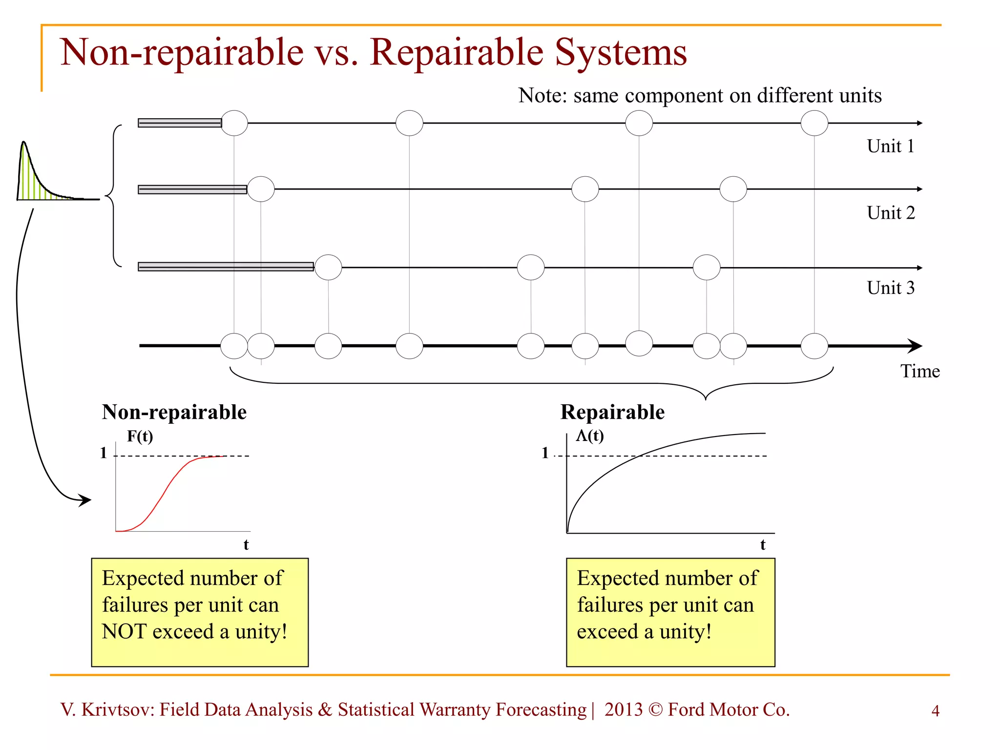
A connection between non-repairable & repairable systems
t
N(t)
E[N(t)]
0
1
2
3
4
5
repair
f(t) = dF(t)/dt – underlying (TTFF)
distribution of non-repairable components
X1 X2 X3 X5X4
])([)()()]([
0
t
NdEtFtFtNE
Fundamental renewal equation:
CumulativeFailures](https://image.slidesharecdn.com/2013asqfielddataanalysisstatisticalwarrantyforecasting-130603174808-phpapp01/75/2013-asq-field-data-analysis-statistical-warranty-forecasting-14-2048.jpg)
![V. Krivtsov: Field Data Analysis & Statistical Warranty Forecasting | 2013 © Ford Motor Co. 14
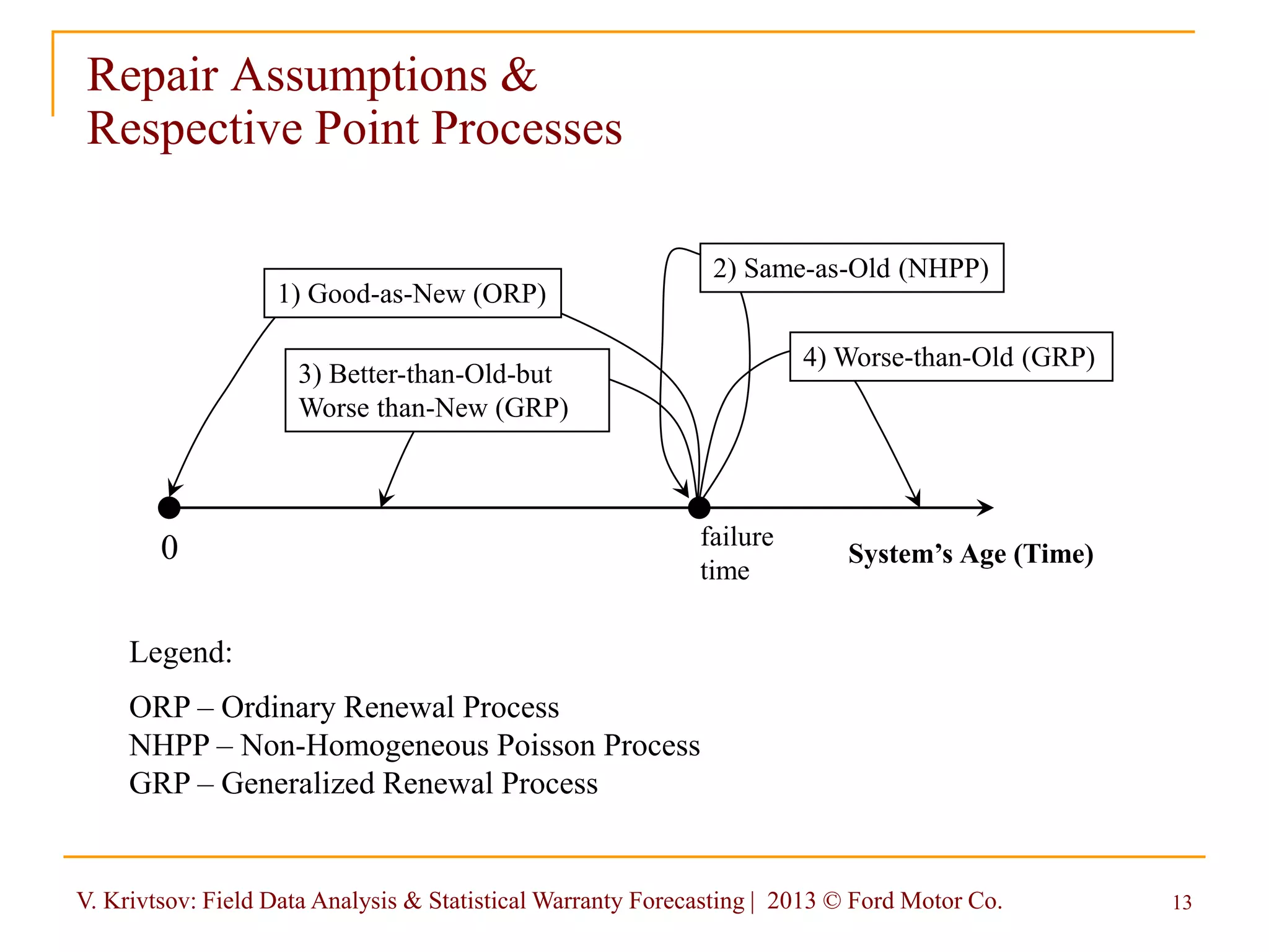
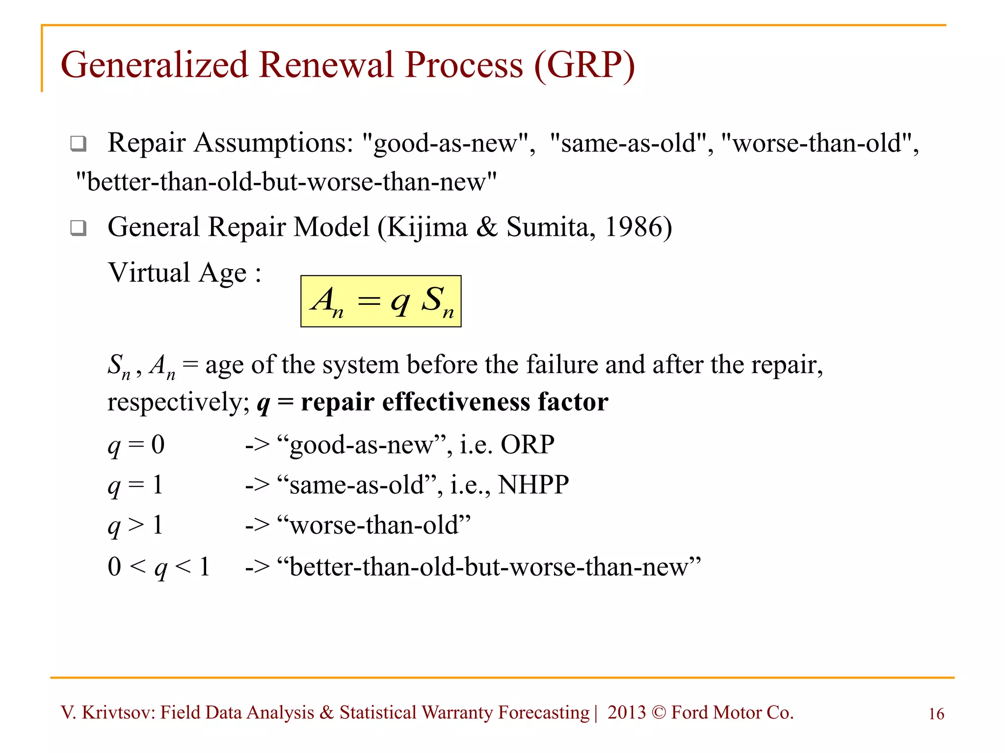
Ordinary Renewal Process
Repair Assumption: “good-as-new”
Expected number of failures in [0, t]:
F(t) = CDF of the time to first failure (TTFF) distribution
Iterative Model (Smith, Leadbetter - 1963)
TTFF distribution: Weibull
Recursive Model (White - 1964)
TTFF distribution: Weibull
Numerical Integration Approach (Baxter, Scheuer - 1982)
TTFF distributions: Weibull, Gamma, lognormal, truncated Gaussian
Pade Approximation Model (Garg, Kalagnanam - 1998)
TTFF distribution: truncated Gaussian
LL
t
dtFtFt
0
)()()()( ](https://image.slidesharecdn.com/2013asqfielddataanalysisstatisticalwarrantyforecasting-130603174808-phpapp01/75/2013-asq-field-data-analysis-statistical-warranty-forecasting-16-2048.jpg)
![V. Krivtsov: Field Data Analysis & Statistical Warranty Forecasting | 2013 © Ford Motor Co. 15
Nonhomogeneous Poisson Process (NHPP)
Repair Assumption: “same-as-old”
Expected number of failures in [0, t]:
l() = the rate of occurrence of failures (ROCOF)
Common Models for l()
Loglinear Model (Cox, Lewis - 1966)
Power Law Model (Crow - 1974)
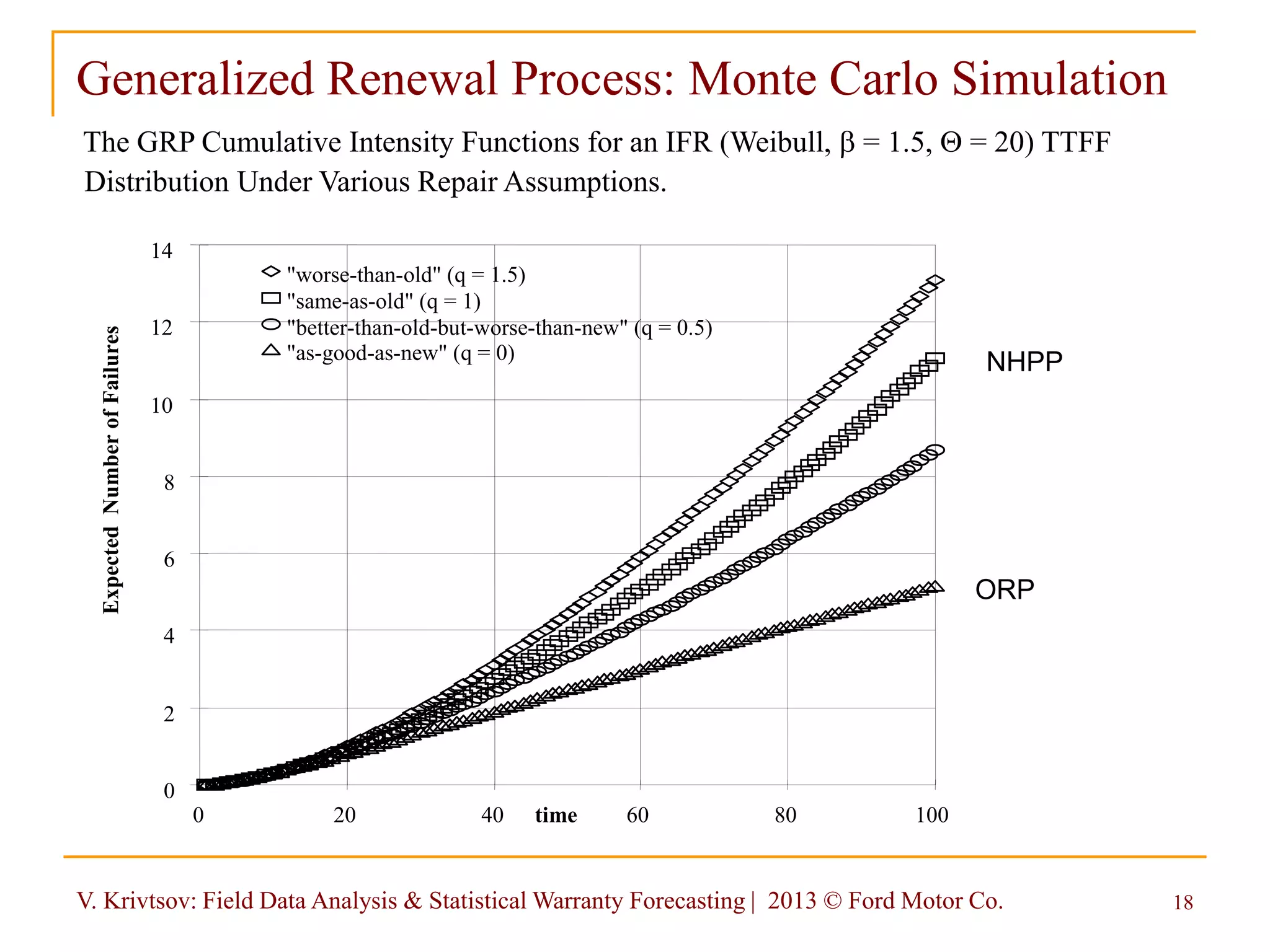
Monte Carlo Simulation
X1 = time to first failure distributed according to F(t),
X2 = time to second failure distributed according to F(t2| X1), where
Failure Interarrival Time
t
0
d)()t( lL
)(
)(
1)|(
1
12
12
XR
XtR
XttF
L
n
i inn XStSnEt 1
)],|[max()(
11
1
)](1[1
iii SStFFX ](https://image.slidesharecdn.com/2013asqfielddataanalysisstatisticalwarrantyforecasting-130603174808-phpapp01/75/2013-asq-field-data-analysis-statistical-warranty-forecasting-17-2048.jpg)
![V. Krivtsov: Field Data Analysis & Statistical Warranty Forecasting | 2013 © Ford Motor Co. 17
Fundamental G-Renewal Equation
Expected number of failures in [0, t]:
where
Closed solution is impossible and numerical solutions via Laplace transform or power series
expansion also fail (Kijima, 1988)
Numerical integration approximations are difficult to apply, because of a recurrent infinite
system issue (Filkenstein, 1997)
A Monte Carlo Solution is, however, possible (Kaminskiy & Krivtsov, 1998)
Failure Interarrival Time
,)|()()0|()(
0 0
ddxxxgxhgt
t
L
0,,
)(1
)(
)(
xt
qXF
qXtf
xtg
L
n
i inn XStSnEt 1
)],|[max()(
1-i
1-i
1-i1-
i Sq,
)SqF(t-1
)SqF(t-1
-1FX
](https://image.slidesharecdn.com/2013asqfielddataanalysisstatisticalwarrantyforecasting-130603174808-phpapp01/75/2013-asq-field-data-analysis-statistical-warranty-forecasting-19-2048.jpg)

![V. Krivtsov: Field Data Analysis & Statistical Warranty Forecasting | 2013 © Ford Motor Co. 26
Weibull Probability Plot: Mechanical Transfuser Data
ReliaSoft Weibull++ 7 - www.ReliaSoft.com
b,,
Time: t
CDF:F(t)
0.100 100.0001.000 10.000
0.001
0.005
0.010
0.050
0.100
0.500
1.000
5.000
10.000
50.000
90.000
99.000
0.001
x 8
x 25
x 46
x 72
x 90
x 88
x 79
x 69
x 86
x 64
0.5
0.6
0.7
0.8
0.9
1.0
1.2
1.4
1.6
2.0
3.0
4.0
6.0
b
Probability-W eibull
CB@ 95% 2-Sided [T]
All Data
W eibull-2P
RRX SRM MED FM
F=627/S=99373
Data Points
Probability Line
Top CB-I
Bottom CB-I
Vasiliy Krivtsov
VVK
9/22/2007
4:51:35 PM
Mechanical Transfuser –
Warranty Forecast Summary:
Failure probability @ 24MIS: 0.1364
Population Size: 110,000
Total Expected Repairs: 15,004
Cost per repair: $30
Total Expected Warranty Cost: $450,120
Year-to-date Cost: $18,810
Required Warranty Reserve: $431,310
13.64
24](https://image.slidesharecdn.com/2013asqfielddataanalysisstatisticalwarrantyforecasting-130603174808-phpapp01/75/2013-asq-field-data-analysis-statistical-warranty-forecasting-28-2048.jpg)

![V. Krivtsov: Field Data Analysis & Statistical Warranty Forecasting | 2013 © Ford Motor Co. 34
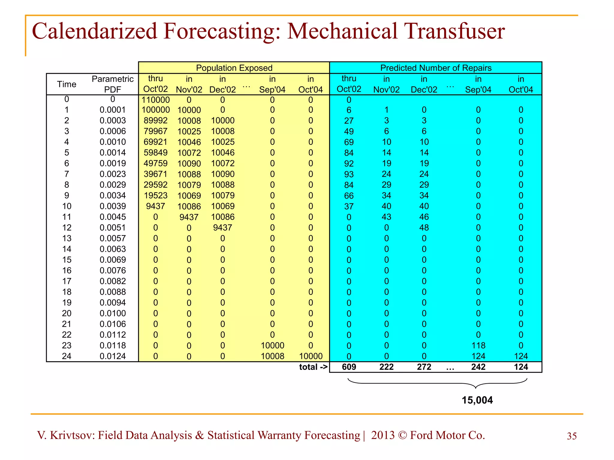
Calendarized Forecasting
ReliaSoft Weibull++ 7 - www.ReliaSoft.com
b,,
Time: t
CDF:F(t)
0.100 100.0001.000 10.000
0.001
0.005
0.010
0.050
0.100
0.500
1.000
5.000
10.000
50.000
90.000
99.000
0.001
x 8
x 25
x 46
x 72
x 90
x 88
x 79
x 69
x 86
x 64
0.5
0.6
0.7
0.8
0.9
1.0
1.2
1.4
1.6
2.0
3.0
4.0
6.0
b
Probability-W eibull
CB@ 95% 2-Sided [T]
All Data
W eibull-2P
RRX SRM MED FM
F=627/S=99373
Data Points
Probability Line
Top CB-I
Bottom CB-I
Vasiliy Krivtsov
VVK
9/22/2007
4:51:35 PM
13.64
24
Mechanical Transfuser –
Warranty Forecast Summary:
Failure probability @ 24MIS: 0.1364
Population Size: 110,000
Total Expected Repairs: 15,004
Cost per repair: $30
Total Expected Warranty Cost: $450,120
Year-to-date Cost: $18,810
Required Warranty Reserve: $431,310
How will this total number of repairs be
distributed along the calendar time, i.e.
how many repairs to expect next month,
the following month, etc.?](https://image.slidesharecdn.com/2013asqfielddataanalysisstatisticalwarrantyforecasting-130603174808-phpapp01/75/2013-asq-field-data-analysis-statistical-warranty-forecasting-36-2048.jpg)
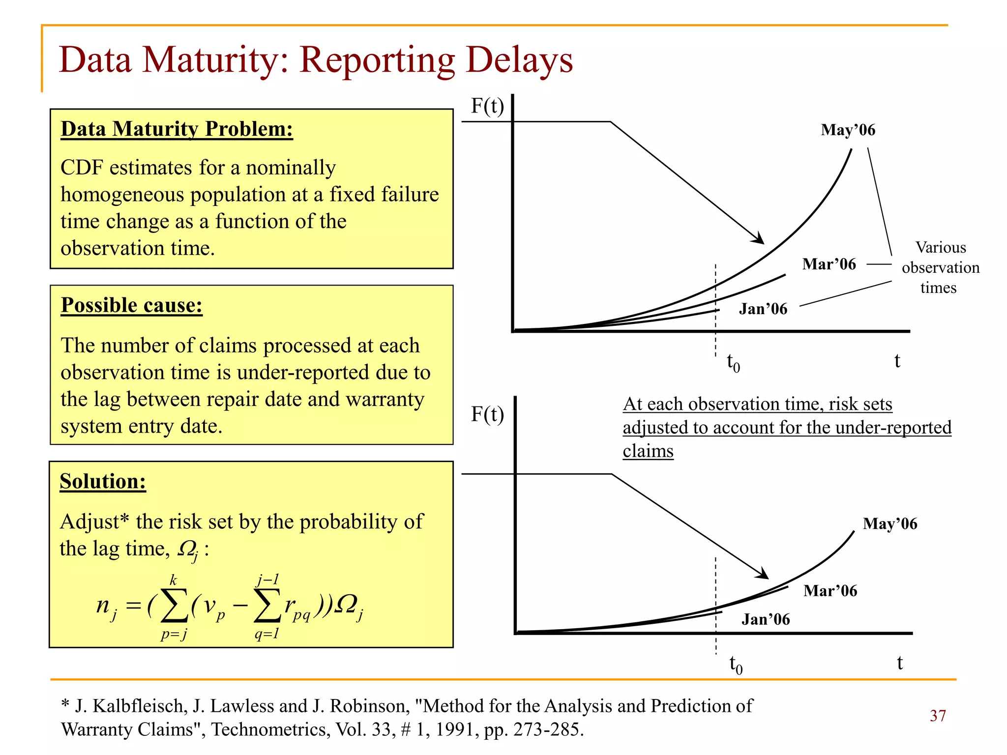
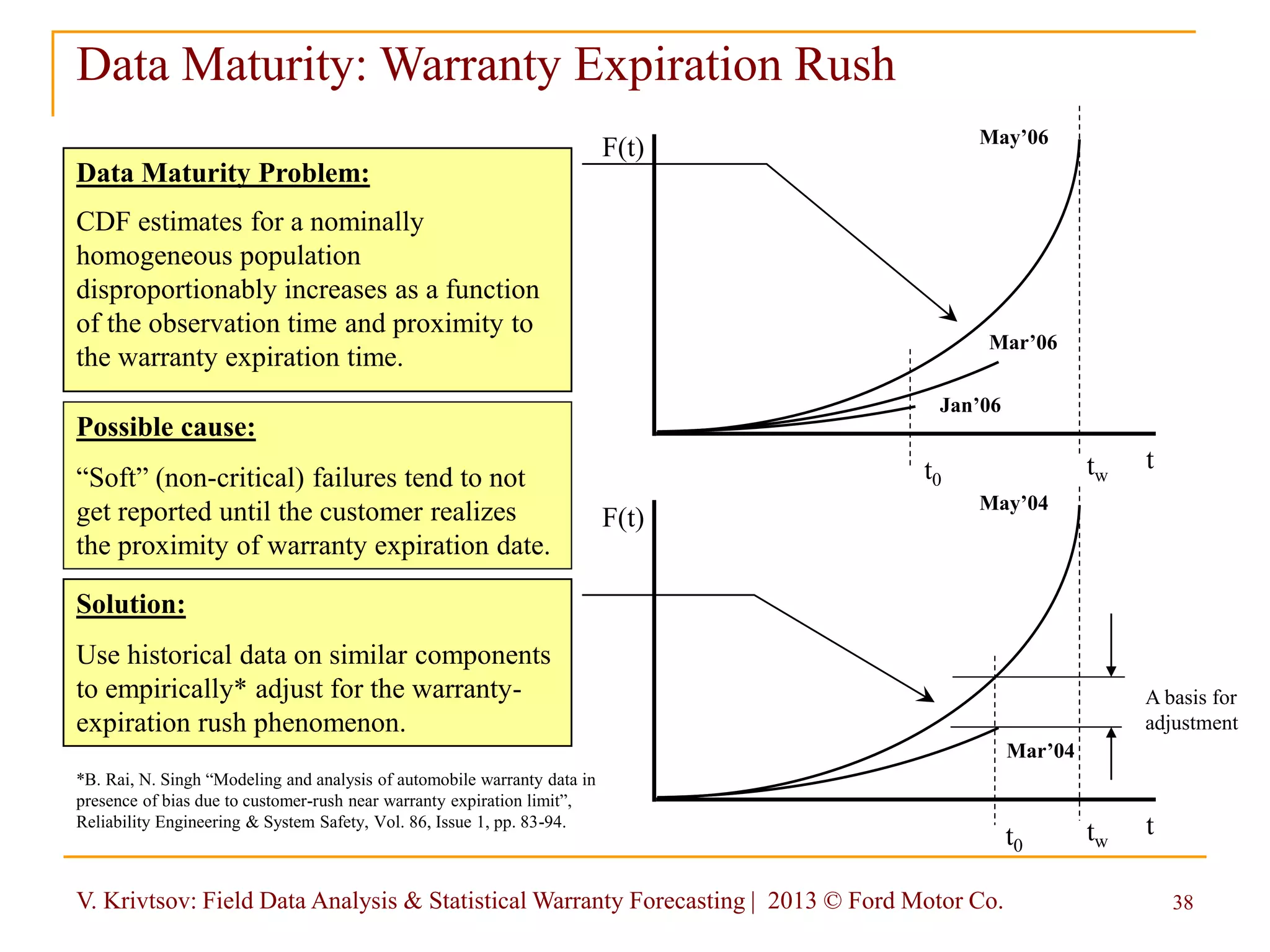

The document discusses field data analysis and statistical warranty forecasting, focusing on probabilistic models for both non-repairable and repairable systems. It addresses key concepts like hazard functions, statistical estimation, and field data maturity issues, along with their significance in managing warranty reserves and optimizing cash flow. The insights presented aim to enhance failure avoidance and cost management through effective data analysis techniques.