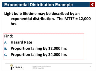
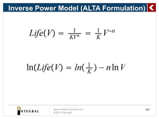
Predicting product life using reliability analysis methods

Predicting Product
Predicting Product
Life Using Reliability
Life Using Reliability
y
Analysis Methods
Steven Wachs
©2011 ASQ & Presentation Steven
Presented live on Nov 09th ~ 11th, 2012

http://reliabilitycalendar.org/The_Re
liability_Calendar/Short_Courses/Sh
liability Calendar/Short Courses/Sh
ort_Courses.html

ASQ Reliability Division
ASQ Reliability Division
Short Course Series
Short Course Series
One of the monthly webinars
One of the monthly webinars
on topics of interest to
reliability engineers.
To view recorded webinar (available to ASQ Reliability
Division members only) visit asq.org/reliability
) /

To sign up for the free and available to anyone live
webinars visit reliabilitycalendar.org and select English
Webinars to find links to register for upcoming events

http://reliabilitycalendar.org/The_Re
liability_Calendar/Short_Courses/Sh
liability Calendar/Short Courses/Sh
ort_Courses.html

Predicting Product Life
Using Reliability Analysis
Methods
Steven Wachs
Principal Statistician
Integral Concepts, Inc.
www.integral-concepts.com
248-884-2276
www.integral-concepts.com 1
©2012 Copyright

Agenda

 Reliability Concepts & Reliability Data
 Probability, Statistics, and Distributions
 Assessing & Selecting Models
 Estimating Reliability Statistics
 Systems Reliability
 Reliability Test Planning
 Accelerated Life Testing
 Warranty Analysis

©2012 Copyright

Motivation

Intense Global Competition

Customer Expectations

Customer Loyalty

Product Liability

©2012 Copyright

Defining Reliability

Reliability is the probability that a
material, component, or system will
perform its intended function under
defined operating conditions for a
specified period of time.

©2012 Copyright

Ambiguity in Definition

 What is the intended function?
 What are the defined operating
conditions?
 How should time be defined?

We must clearly define these characteristics
when defining reliability for a specific
application
©2012 Copyright

Reliability Data

 Life Data
 Time-To-Failure (TTF) Data
 Time-Between-Failure (TBF) Data
 Survival Data
 Event-time Data
 Degradation Data

©2012 Copyright

Unique Aspects of Reliability Data

 Presence of Censoring
 Reliability Models based on positive
random variables (e.g. exponential,
lognormal, Weibull, gamma)
 Interpolation and extrapolation often
required

©2012 Copyright

Repairable vs. Non-repairable

 The focus of this course is non-
repairable components or systems
(characterized by time to failure)

 Repairable systems are characterized
by time between failure

©2012 Copyright

The Bathtub Curve

©2012 Copyright

The Reliability Function

R(to ) = P(T > to )

where T =“time”
to failure

©2012 Copyright

Censored Data

 When exact failure times are not known

 Provides useful information for estimation
of reliability (Do NOT drop from analysis)

 Types of Censoring
– Right Censoring
– Left Censoring
– Interval Censoring

©2012 Copyright

Types of Censoring
Left Censoring Right Censoring

Interval Censoring

©2012 Copyright

Other Censoring Ideas

 Competing Risks

• Impact on Reliability estimates
• Alternatives (if extreme censoring exists)
– Use Accelerated Testing Conditions
– Use Degradation Data

©2012 Copyright

Agenda


©2012 Copyright

Describing Time to Failure

©2012 Copyright

Integrating the PDF

B

c fxdx
d
PX  B  PX  c, d 
©2012 Copyright

Reliability
Distribution Plot
0.0008

0.0007

0.0006

0.0005
Density

0.0004

0.0003

0.0002

0.0001 R(1500)

0.0000
0 1500
X

©2012 Copyright

Failure Probability (Cumulative)
Distribution Plot
0.0008
F(500)
0.0007

0.0006

0.0005
Density

0.0004

0.0003

0.0002

0.0001

0.0000
0 500
X

©2012 Copyright

The CDF

 fxdx
t
Ft  PX  , t 

©2012 Copyright
19

CDF/Reliability Relationship

©2012 Copyright

Hazard Function (Rate)

The propensity to fail in the next instant
given that it hasn’t failed up to that
time (“instantaneous failure rate
function”)

ft ft
ht  1Ft
 Rt

©2012 Copyright

Mean Time to Failure (MTTF)

 The Expected Value or the Mean of the Time
to Failure Random Variable
 The average time to failure (often
significantly larger than the median time to
failure)
 The MTTF can be misleading as often as
much as 70% of the population will fail
before the MTTF
 
MTTF  ET  0 tftdt  0 Rtdt
©2012 Copyright

B-Life (or Quantile)

The time at which a
specified proportion
of the population is
expected to fail

©2012 Copyright

Advantages of Parametric Models
 May be described concisely with a few
parameters

 Allows extrapolation (in time)

 Provide “smooth” estimates of failure
time distributions

©2012 Copyright

Common Distributions in Reliability

 Weibull
 Exponential
 Lognormal
 Gamma
 Binomial
 Loglogistic
 Etc.

©2012 Copyright

Exponential Distribution

 The simplest model used in reliability
analysis (and sometimes misused)

 Described by a single parameter, l which
is the hazard rate (inverse of MTTF)

 Key property: the hazard rate is constant
(the only distribution with this property)

©2012 Copyright

Exponential Distribution

• pdf: f(t) = le-lt
• cdf: F(t) = 1 - e-lt
• Reliability: R(t) = e-lt
• Hazard rate: h(t) = l
• MTTF = 1/l = q
• Quantile: F-1(p) = (1/l)[-ln(1-p)]

©2012 Copyright

Exponential Distribution Example

Light bulb lifetime may be described by an
exponential distribution. The MTTF = 12,000
hrs.

Find:
A. Hazard Rate
B. Proportion failing by 12,000 hrs
C. Proportion failing by 24,000 hrs

©2012 Copyright

Exponential Distribution Example

Solution
A. l = 1/12,000 = 0.000083 = 83 failures per
million hrs
12,000
B. F12, 000  1  e 12,000  1 1
e  0. 632
24,000
C. F24, 000  1  e 12,000  1 1
 0. 865
e2

©2012 Copyright

Exponential Distribution Guidelines

 Constant hazard rate implies that the
probability that a unit will fail in the next
instant does not depend on the unit’s age

 Reasonable for many electronic
components that do not wear out

 Usually inappropriate for modeling TTF of
mechanical components that are subject
to fatigue, corrosion, or wear
©2012 Copyright

The Weibull Distribution

 The most common model in reliability analysis

 Described by 2 parameters:
h = “scale” parameter
b = “shape” parameter

 Flexible model that can effectively model a
wide variety of failure distributions

©2012 Copyright

The Weibull Distribution (some functions)

 1  t 
 pdf: ft     t
 e 


 t
 cdf: Ft  1  e 


 t
 Reliability: Rt  e 

 1
 Hazard rate: ht     t


©2012 Copyright

The Weibull Shape Parameter

Failure Rate

?

©2012 Copyright

The Weibull Scale Parameter

?

©2012 Copyright

Weibull Characteristics

 h is also referred to as the 63.2nd
percentile
 To see this: set t = h in F(t)
 

Ft  F  1  e 

1 
 1e
 1  e  0. 632
1

• The value of b is irrelevant when t =
h
©2012 Copyright

Conditional Reliability

 An application of conditional probability
 Needed to estimate reliability when “burn-
in” is used or to estimate reliability after a
warranty period.

Rtt 0 
Rt|t 0   Rt 0 
©2012 Copyright

Agenda


©2012 Copyright

Selecting Models

 Given time-to-failure data (failures and
censored data), which distribution best
describes the data?
 Graphical Methods (probability
plotting) and/or Statistical Methods
may be utilized

©2012 Copyright

Probability Plots

 Graphical method to assess “fit”
 Fit is determined by how well the plotted
points align along a straight line
 Plotted variables are “transformed” so that
y is a linear function of x
– X axis: Plot observed failure times
– Y axis: Plot estimated cumulative probabilities
(p)

©2012 Copyright

Probability Plotting

©2012 Copyright

Constructing Probability Plots
• X-Axis – Observed/Transformed
Failure Times

• Y-Axis – Estimated/Transformed
Cumulative Probabilities

• Transformed quantities for plot
depend on the distribution

©2012 Copyright

Constructing Probability Plots

©2012 Copyright

Linearizing the CDF - Example

 Consider the Weibull distribution. Recall
that the Weibull cdf is:

 t
Ft  1  e 

• We need to transform F(t) to achieve
a linear function

©2012 Copyright

Linearizing the CDF - Example

 t
1  Ft  e 

t 
1
1Ft
e 


ln 1Ft     
1 t

ln ln 1Ft 
1
  lnt   ln

By setting: y  ln ln 1Ft 
1

x  lnt
C   ln
we have: y  x  C

©2012 Copyright

Graphical Estimation

2.75
b = 2.0/2.75
= 0.73

2.0

h

©2012 Copyright

Selecting Models
 Multiple Distributions may adequately
describe the time-to-failure data
 Sensitivity Analysis is recommended
to assess how reliability predictions
vary with alternative viable models
 Confidence Intervals on reliability
estimates do not include model
uncertainty

©2012 Copyright

Selecting a Distribution

©2012 Copyright

Handling Multiple Failure Modes

 Multiple Failure Modes should be
modeled separately (if data exists)
 Failure rates of the various failure
modes are typically different
 Overall Reliability may be predicted
using system reliability concepts
(series model)

©2012 Copyright

ReliaSoft Weibull++ 7 - www.ReliaSoft.com
Probability - W eibull
99.000
Probability-Weibull

Data 1
Weibull-2P
90.000 ML E SRM MED FM
F=40/S=0
Data Points
Probability Line

50.000
U n re l i a b i l i ty , F (t)

10.000

5.000

Steven Wachs
integral Concepts, Inc.
10/28/2011
1:05:27 PM
1.000
0.010 0.100 1.000 10.000 100.000 1000.000 10000.000
Time, ( t)
b   h    

©2012 Copyright

Probability - W eibull
99.000
Probability-Weibull

Data 1
Weibull-CFM
90.000 ML E SRM MED FM
CFM 1 Points
CFM 2 Points
CFM 1 L ine
CFM 2 L ine
Probability Line

50.000
U n re l i a b i l i ty , F (t)

10.000

5.000

Steven Wachs
10/28/2011
1:03:08 PM
1.000
0.010 0.100 1.000 10.000 100.000 1000.000 10000.000
Time, ( t)
b    h      b   h  

©2012 Copyright

Agenda


©2012 Copyright

Reliability Estimation

 From the time-to-failure distribution we
can estimate quantities like:
• Reliability at various times
• Time at which x% are expected to fail
• Failure (hazard) rates
• Mean time to failure

 Confidence Intervals or Bounds should
be included to account for estimation
uncertainty
©2012 Copyright


 Estimation Methods
• Maximum Likelihood Estimation (MLE):
nice statistical properties, handles
censored data well, biased estimates for
small sample sizes

• Rank Regression: Unbiased estimates but
poorer precision and does not handle
censored data as well as MLE

©2012 Copyright

Properties of Estimators

 Bias – The extent to which the estimator
differs on average from the true value. (An
unbiased estimator equals the true value
on average)

 Precision – The amount of variability in the
estimates.

©2012 Copyright

Properties of Estimators

©2012 Copyright

Estimation Methods

 Maximum Likelihood Estimation
– Generally preferred by statisticians (minimum
variance) although the estimates tend to be biased

– ML method finds parameter values which maximize
the likelihood function (the joint probability of
observing all of the data).

– The maximization of the likelihood function usually
must be done numerically (rather than
analytically).

©2012 Copyright

MLE Example (Weibull)
• Given failure time data, we need to
estimate h, b.
i1 fx i  fx 1 fx 2 . . . fx n 
n
L

L      e
n  x 1  xi
i 
i1

• We maximize likelihood function by
taking derivatives with respect to
each parameter

©2012 Copyright

Effect of Censored Data on the Likelihood Function

• With no censoring, the likelihood
function is:

i1 fx i   fx 1 fx 2 . . . fx n 
n
L

• Censored observations cannot
use the pdf since the failure
time is unknown

©2012 Copyright


• Suppose we have a right-censored
observation at time = 1500?

• What function indicates the probability of
this occurring?

©2012 Copyright


• Suppose we have a right-censored

this occurring?

• R(1500) gives the probability that a unit fails
at time 1500 or later.

©2012 Copyright


Distribution Plot
0.0008

0.0007

0.0006

0.0005
Density

0.0004

0.0003

0.0002

0.0001 R(1500)

0.0000
0 1500
X

©2012 Copyright


• Suppose we have a left-censored

this occurring?

©2012 Copyright


• Suppose we have a left-censored observation
at time = 500?

this occurring?

• F(500) gives the probability that a unit fails at
time 500 or earlier.

©2012 Copyright


Distribution Plot
0.0008
F(500)
0.0007

0.0006

0.0005
Density

0.0004

0.0003

0.0002

0.0001

0.0000
0 500
X

©2012 Copyright


• Suppose we have an interval censored
condition where the failure occurred
between 1000 and 1300.

this occurring?

©2012 Copyright


• Suppose we have an interval censored
condition where the failure occurred
between 1000 and 1300.

this occurring?

• F(1300)-F(1000) gives the probability that a
unit fails between 1000 and 1300

©2012 Copyright


Distribution Plot
0.0008

0.0007

0.0006

0.0005 F(1300)-F(1000)
Density

0.0004

0.0003

0.0002

0.0001

0.0000
0 1000 1300
X

©2012 Copyright

Estimation Methods

• Rank Regression
– Determines best fit line on the probability
plot by using least squares regression

– Fitted line is used to estimate parameters

©2012 Copyright

Failure Probability Plot

©2012 Copyright

Estimating with Multiple Failure Modes
Failure Time Failure Model Failure Time Failure Model
63 linkage 791 motor
384 linkage 874 linkage
485 motor 999 motor
655 motor 1299 motor
662 linkage 1481 linkage

©2012 Copyright

Linkage Failure Mode
Distribution Analysis: Failure Time

Variable: Failure Time
Failure Mode: fm = linkage

Censoring Information Count
Uncensored value 20
Right censored value 20

Estimation Method: Maximum Likelihood

Distribution: Weibull

Parameter Estimates

Standard 95.0% Normal CI
Parameter Estimate Error Lower Upper
Shape 1.34641 0.264909 0.915592 1.97994
Scale 1325.81 240.466 929.169 1891.76

©2012 Copyright

Motor Failure Mode
Distribution Analysis: Failure Time

Variable: Failure Time
Failure Mode: fm = motor

Censoring Information Count
Uncensored value 20
Right censored value 20

Estimation Method: Maximum Likelihood

Distribution: Weibull

Parameter Estimates

Standard 95.0% Normal CI
Parameter Estimate Error Lower Upper
Shape 4.17342 0.634609 3.09784 5.62245
Scale 1154.46 62.7168 1037.86 1284.17
©2012 Copyright

Multiple Failure Modes
Probability Plot for Failure Time
Complete Data - ML Estimates
F ailure M ode = linkage
Failure Mode = linkage Failure Mode = motor S hape S cale
Weibull - 95% CI Weibull - 95% CI 1.34641 1325.81

F ailure M ode = motor
95 95 S hape S cale
4.17342 1154.46
80 80

50 50
Percent

20 Percent 20

5 5

2 2

1 1
10 100 1000 10000 500 1000 2000
Failure Time Failure Time

©2012 Copyright

Survival Plot for Failure Time
F ailure M ode = linkage
Failure Mode = linkage Failure Mode = motor S hape S cale
Weibull - 95% CI Weibull - 95% CI 1.34641 1325.81

F ailure M ode = motor
100 100 S hape S cale
4.17342 1154.46

80 80

60 60
Percent

Percent
40 40

20 20

0 0

0 1500 3000 4500 500 1000 1500
Failure Time Failure Time

©2012 Copyright

Survival Plot for Failure Time
Multiple Distributions - 95% CI

100

80

60
Percent

40

20

0

0 200 400 600 800 1000 1200 1400 1600
Failure Time

©2012 Copyright

Confidence Intervals
• An interval (l, u) around the point estimate that
contains the true value with high probability

• The interval is said to be a P% confidence interval
if P percent of the intervals we might calculate
from replicated studies contain the true
parameter value

©2012 Copyright

Improving Precision of Estimates

 More Data (Failures) = Better Precision
(tighter confidence intervals)
 Can make more assumptions (assume
distribution parameters)
 Reduce confidence level (not a real
solution)

©2012 Copyright

Agenda


©2012 Copyright

System Reliability

 A System may be thought of as a collection of
components or subsystems

 System Reliability Depends on:
a. Component reliability
b. Configuration (redundancy)
c. Time

©2012 Copyright

A Series System

i1 R it  R 1 tR 2 tR 3 tR 4 t
4
R s t 

Example: If the component reliabilities are 0.9, 0.9. 0.8, 0.8 at 1 year
Then the System reliability at 1 year is: 0.9*0.9*0.8*0.8 = 0.52

©2012 Copyright

Series Model for Multiple Failure Modes

n
Rt   R it  R A tR BtR C tR Dt
i1

©2012 Copyright

A Parallel System (Redundant Components)

R s t  1  F s t
 1  F 1 tF 2 tF 3 t
 1  1  R 1 t1  R 2 t1  R 3 t

©2012 Copyright

A Parallel System (Redundant Components)

Example: If the component reliabilities are 0.9, 0.9. 0.9 at 1 year
Then the System reliability at 1 year is: 1 - (.1)*(.1)*(.1) = 0.999

©2012 Copyright

k-out-of-n Parallel Systems
 System consists of n components in which k of
the n components must function in order for
the system to function

 For example, if 2 of 4 engines are required to
fly, then the system will not fail if:
– All 4 engines operate
– Any 3 operate
– Any 2 operate

©2012 Copyright


If all components have the same reliability, R(t):

The probabilities of all possible combinations leading to success are
summed

©2012 Copyright

k-out-of-n Parallel Systems Example

Suppose a system consists of 6 identical pumps. For the
system to function, at least 4 of the 6 pumps must operate. If
the reliability of each pump at 3 years in service is 0.90, what
is the system reliability at 3 years?

©2012 Copyright

Effect of k on System Reliability

 As k increases, system reliability decreases

 If k = 1 Pure Parallel System

 If k = n Series System

©2012 Copyright

Effect of k on System Reliability
System Reliability vs k (k-out-of-6, R = 0.90)

1.0

0.9

0.8 k Reliability
Reliability

1 1.0000
2 0.9999
0.7 3 0.9987
4 0.9842
5 0.8857
0.6 6 0.5314

0.5
1 2 3 4 5 6
k

©2012 Copyright

 When the components in the k-out-of-n
parallel configuration do not share the same
reliability function, all possible combinations
must be computed

 Example follows

©2012 Copyright

k-out-of-n System Example

Three generators are
configured in parallel. At 0.90
least two of the
generators must
function in order for the 0.8 2/3
system to function. At 5 7
years: R1 = 0.90, R2 =
0.87, R3 = 0.80. What is 0.80
the System Reliability at
5 years?

©2012 Copyright

 Here, k = 2, n = 3

 The following combinations of events lead to a
reliable system at 5 years in service:
– generator 1,2 operate and generator 3 fails
– All three generators operate

©2012 Copyright


R1 = 0.90
R2 = 0.87
R3 = 0.80
©2012 Copyright

Reliability Block Diagrams

Used to Model System and
Estimate System Reliability

©2012 Copyright

Reliability Allocation Problems

Given a reliability target for the system, how
should subsystem and/or component level
reliability requirements be established so that the
system objective is met?

Typical Goals
a. Maximize the System Reliability for a given cost
b. Minimize the Cost for a given System Reliability

Improve component reliability or add
redundancies?

©2012 Copyright

Agenda


©2012 Copyright

Reliability Test Planning

 Estimation Test Plans
 Determine sample size needed to
estimate reliability characteristics with a
specified precision

 Planning information such as assumed
distribution parameters, testing time, and
censoring scheme is required

 Failures during testing are required

©2012 Copyright

Sample Sizes for Desired
Precision
 We select sample size to achieve the desired
precision in our estimates

 Larger sample size  Greater precision

 Greater precision  Smaller confidence
intervals

©2012 Copyright

Sample Size Calculations

Calculation Depends On:
 Distribution used to model the failure data
 Level of precision desired
 Confidence level
 Presence of censoring
 Length of test (for Type I censoring)
 Failure proportion (for Type II censoring)

©2012 Copyright

Estimation Test Plan
Type I right-censored data (Single Censoring)

Estimated parameter: 50th percentile
Calculated planning estimate = 124.883
Target Confidence Level = 95%

Planning distribution: Weibull
Scale = 150, Shape = 2

Actual
Censoring Sample Confidence
Time Precision Size Level
100 62.435 8 96.2010

©2012 Copyright

Reliability Test Planning

 Demonstration Test Plans
 Determine sample size (or testing time)
needed to demonstrate reliability
characteristics (e.g. lower bound on
reliability)

 Planning information such as assumed
distribution and parameter is required

 Failures during testing are not required

©2012 Copyright

Reliability Demonstration

 Evaluates the following hypothesis
H0: The reliability is less than or equal to a
specified value

H1: The reliability is greater than a specified
value

©2012 Copyright

Types of Test Plans

 Zero-Failure Test Plans
– Test demonstrates reliability if zero failures
are observed during test
– Useful for highly reliable items

 M-Failure Test Plans
– Test demonstrates reliability if no more
than m failures occur
– Permit verification of test design
assumptions
©2012 Copyright

Planning Information

 Assumptions needed:
– Distribution
– Shape Parameter (for Weibull)
– Scale Parameter (for other distributions such
as lognormal, loglogistic, logistic, extreme
value)
– Assumptions based on expert opinions, prior
studies, similar products
– Sensitivity analysis is recommended

©2012 Copyright

Computing Test Time or Sample Size

 We specify either the sample size or the
testing time allocated for each unit (the
other quantity is computed)

 Demonstration Test Plan consists of:
– The maximum number of failures allowed
– The sample size
– The testing time for each unit

©2012 Copyright

Example: Demonstration Test Plan

 Reliability Goal: 1st percentile > 80,000 mi

 TTF estimated by Weibull w/ b = 2.5

 Can test for 120,000 miles

 How many units are needed for zero-failure
and 1-failure test plans?
©2012 Copyright


Demonstration Test Plans

Reliability Test Plan
Distribution: Weibull, Shape = 2.5
Percentile Goal = 80000,Target Confidence Level = 95%

Actual
Failure Testing Sample Confidence
Test Time Size Level
0 120000 108 94.9768

©2012 Copyright



Percentile Goal = 80000,Target Confidence Level = 95%

Actual
1 120000 172 95.0241

©2012 Copyright


 Suppose we can only test 50 units?
Percentile Goal = 80000,Actual Confidence Level = 95%

Failure Sample Testing
Test Size Time
0 50 163392

©2012 Copyright

Probability of Passing (POP)
Likelihood of Passing for Weibull Model
Maximum Failures = 0, Target Alpha = 0.05
Time = 120000, N = 108, Actual alpha = 0.0502316

100

80

60
Percent

40

20

0

2 4 6 8 10
Ratio of Improvement

©2012 Copyright

Probability of Passing (POP)
Likelihood of Passing for Weibull Model
Maximum Failures = 1, Target Alpha = 0.05
Time = 120000, N = 172, Actual alpha = 0.0497587

100

80

60
Percent

40

20

0

2 4 6 8 10
Ratio of Improvement

©2012 Copyright

Demonstration Test Plan (1st Percentile)
Percentile Goal = 80000, Target Confidence Level = 95%

Actual
0 120000 108 94.9768
1 120000 172 95.0241
2 120000 228 94.9669
3 120000 281 94.9567

©2012 Copyright

Test Units vs Test Time
772.775
0 Failures
1 Failures
2 Failures
3 Failures

639.853

506.932
N u m b e r o f T e s t U n i ts

374.010

241.088

Steven Wachs
10/28/2011
2:25:16 PM
108.167
80000.000 88000.000 96000.000 104000.000 112000.000 120000.000
Test Time

©2012 Copyright

Agenda


©2012 Copyright

Introduction to ALT
 Purpose:To estimate reliability on a
timely basis

 Inducefailures sooner by testing at
accelerated stress conditions

 Extrapolateresults obtained at
accelerated conditions to use conditions
(using acceleration models)

 Focus
on one or a small number of failure
modes
©2012 Copyright

ALT Models (2 parts)

©2012 Copyright

Life is a Function of Time and Stress

©2012 Copyright

Life-Stress Relationship
ReliaSoft AL TA 7 - www.ReliaSoft.com
Lif e vs Stress
100000.000
Life

Data 1
Ey ring
Weibull
323
F=30 | S=0
Eta L ine
1%
99%
393
Stress Lev el Points
Eta Point
Imposed Pdf
408
Eta Point
Imposed Pdf
423
Eta Point
Imposed Pdf
L i fe

10000.000

Steven Wachs
7/7/2011
3:07:17 PM
1000.000
300.000 328.000 356.000 384.000 412.000 440.000
Temperature
Beta=4.2918; A=-11.0878; B=1454.0864

©2012 Copyright

Accelerated Stress Testing

 Combination of Statistical Modeling and
understanding of Physics of Failure
 Care must be taken in designing tests to
yield useful information
 ALT models should be refined based on
correlation to actual results obtained at
normal use conditions

©2012 Copyright

Accelerated Life Testing - Topics
 Purpose and Key Concepts

 Accelerated Life Test Models

 One, Two, and Multiple Stress Models

 ALT Test Planning

 Accelerated Degradation Models

 Pitfalls, Guidelines, and Examples
©2012 Copyright

Introduction to ALT
 Purpose: To estimate reliability on a timely
basis

 Induce failures sooner by testing at accelerated
conditions

 Extrapolate results obtained at accelerated
conditions to use conditions (using acceleration
models)

 Focus on one or a small number of failure
modes
©2012 Copyright

Types of Accelerated Testing
– Units tested until failure
– Accelerating factor(s) are used to shorten the
time to failure

 Accelerated Degradation Testing
– Accelerating factor(s) are used to promote
degradation
– Amount of degradation observed during test
– Degradation data used to predict actual time
to failure at stressed conditions
©2012 Copyright

Accelerating Methods

1. Increase Usage Rate
– Increase usage rate from normal usage rate
– ex. Car door hinges have median lifetime of
44,000 cycles (15 years at 8 cycles per day)
– Increasing rate to 5000 cycles per day will
reduce median lifetime to 9 days.
– Assumes TTF is independent of usage rate
– Need to avoid unintended “stress” (e.g.
temp) caused by higher usage rate

©2012 Copyright

Accelerating Methods
2. Test Under Stress Conditions
• Test at higher levels of one or multiple stress
factors
• Common stress factors
– temperature
– thermal cycling
– voltage
– pressure
– mechanical load
– humidity

©2012 Copyright

Types of Stress Loading

©2012 Copyright

Accelerated Life Test Models
ALT Models have 2 parts
1. Stochastic Part
• failure time distribution at each level of
stress
• Use distribution fitting to fit appropriate
models (Weibull, lognormal, etc.) at each
level of stress

2. Structural Part
• Life-stress relationship
• Use regression models to relate the stress
variable to the Time To Failure Distribution
©2012 Copyright

ALT Models have 2 parts

©2012 Copyright

Acceleration Models

 Acceleration models relate accelerating
factors (e.g. temp, voltage) to the TTF
distribution.

 Model depends on acceleration method
(usage or stress) and the type of stress

 Physical models are based on physical or
chemical theory that describes the failure
causing process
©2012 Copyright

Life-Stress Models
 Increased stress promotes earlier failures and
life is predicted as a function of time and stress

 Common stress factors include:
– Temperature, Load, Pressure, Voltage, Current,
Thermal cycling, etc.

 The models assume stress levels are positive.
For temperature, use absolute temperature
(Kelvin) instead of Celsius or Farenheit

©2012 Copyright

Acceleration Factor

 Quantifies the degree to which a given
stress accelerates failure times

AF = Life at Use Condition / Life at Stress Condition

 Acceleration factor increases with stress

©2012 Copyright

Acceleration Factor
ReliaSoft ALTA 7 - www.ReliaSoft.com
Acc el erati on Factor vs Stres s
10.000
Acceleration Factor

Data 1
Arrhenius
Weibull
323
F= | S=
30 0
AF Line
8.000
A c c e le r a t io n F a c t o r

6.000

4.000

2.000

Steven Wachs
8/17/2011
9:47:29 PM
0.000
300.000 340.000 380.000 420.000 460.000 500.000
Temp erat u re
Beta=4.2916; B=1861.6187; C=58.9848

©2012 Copyright

Arrhenius Model (Temp Acceleration)

 Commonly used for products which fail as
a result of material degradation at
elevated temperatures

 Based on a kinetic model that describes
the effect of temperature on the rate of a
simple chemical reaction.

©2012 Copyright

Arrhenius Relationship

Rate = rate of a chemical reaction (rate is inversely
proportional to life)
tempK = absolute temperature in the Kelvin scale
= temp in deg C + 273.15
kB = Boltzmann’s constant = 8.6171x10-5= 1/11605
electron volts per deg C
Ea = activation energy in electron volts
g = a constant
(Ea and g are product or material characteristics)
©2012 Copyright

Arrhenius Model (ALTA Formulation)

Rate = rate of a chemical reaction (rate is inversely
proportional to life)
T = absolute temperature in Kelvin
kB = Boltzmann’s constant = 8.6171x10-5= 1/11605
electron volts per deg C
Ea = activation energy in electron volts
C = a constant

©2012 Copyright

Arrhenius Model (ALTA Formulation)

Let:

Then:

©2012 Copyright

Arrhenius-Weibull Model

The Weibull PDF

Scale Parameter

b, B, and C are estimated from the data (MLE)
(the PDF is a function of time and temperature)

©2012 Copyright

Inverse Power Law Model

 Supports a variety of stress variables such as
voltage, temperature, load, etc.

 Assumes that the product life is proportional
to the inverse power of the stress induced

©2012 Copyright

Inverse Power Law Relationship

where:
T(V) = TTF at a given voltage
V = Voltage
A = constant (product characteristic)
a = constant (product characteristic)
(Voltage is the acceleration variable here)

©2012 Copyright

Inverse Power Model (ALTA Formulation)

Taking logs of both sides, we have:

If failure time and stress are on log scales, this is a linear relationship

©2012 Copyright

Other Models

 Some 2-stress and multiple stress models
will be mentioned later

 Many specific models have been developed
(for certain materials, failure modes, and
applications) although most may be
modeled with general formulations.

©2012 Copyright

Guidelines for ALT Models
 Acceleration Factor(s) should be chosen to
accelerate failure modes
 The amount of extrapolation between test stresses
and use condition should be minimized
 Different failure modes may be accelerated at
different rates (best to focus on one or two modes)
 The available data will generally provide little
power to detect model lack of fit. An
understanding of the physics is important.

©2012 Copyright

Guidelines for ALT Models
 Sensitivity analysis should be performed to assess
the impact of changing model assumptions
 ALT should be planned and conducted by teams
including personnel knowledgeable about the
product, its use environment, the
physical/chemical/mechanical aspects of the
failure mode, and the statistical aspects of the
design and analysis of reliability tests
 ALT results should be correlated with longer term
tests or field data

©2012 Copyright

Strategy for Analyzing ALT Data
1. Examine the data graphically
2. Generate multiple probability plots
3. Fit an overall model
4. Perform residual analysis
5. Assess reasonableness of the model
6. Utilize model for predictions (with
uncertainly quantified)

©2012 Copyright

Example – Analyzing ALT Data
 ALT of mylar-polyurethane insulation used
in high performance electromagnets*
 Insulation has a characteristic dielectric
strength which may degrade over time
 When applied voltage exceeds dielectric
strength a short circuit will occur
 Accelerating variable is voltage

*From Meeker & Escobar (1998)

©2012 Copyright

Time to Failure (Minutes) of Mylar-Polyurethane Insulation

Voltage Stress (kV/mm)
219.0 157.1 122.4 100.3

15.0 49.0 188.0 606.0
16.0 99.0 297.0 1012.0
36.0 154.5 405.0 2520.0
50.0 180.0 744.0 2610.0
55.0 291.0 1218.0 3988.0
95.0 447.0 1340.0 4100.0
122.0 510.0 1715.0 5025.0
129.0 600.0 3382.0 6842.0
625.0 1656.0
700.0 1721.0

©2012 Copyright

• TTF data collected at four stress (voltage)
levels

• Normal operating voltage level is 50 kV/mm

• Fit appropriate model

• Find 95% confidence interval for the B10 life

©2012 Copyright

Graphical Analysis

©2012 Copyright

Multiple Probability Plots

©2012 Copyright

Finds the best fitting stochastic model given
a specified structural model

©2012 Copyright

Fitting the Model

Model: Inverse Power Law
Std. = scale parameter for Distribution: Lognormal
Lognormal distribution Analysis: MLE
Std: 1.049793128
The location parameter
is a function of Voltage K: 1.149419255E-012
per the IPL model n: 4.289109625
LK Value: -271.4247009
Fail Susp: 36 0
©2012 Copyright

Probabi l i ty - Lognormal
99.000
Probability

Data 1
Inverse Power Law
Lognormal
100.3
F= | S=
8 0
Stress Level Points
Stress Level Line
122.4
F= | S=
8 0
Stress Level Points
Stress Level Line
157.1
F= | S=
10 0
Stress Level Points
Stress Level Line
219
F= | S=
10 0
U n r e lia b ilit y

Stress Level Points
Stress Level Line
50
50.000 Use Level Line

10.000

5.000

Steven Wachs
8/19/2011
3:15:43 PM
1.000
10.000 100.000 1000.000 10000.000 100000.000
Time
Std=1.0498; K=1.1494E-12; n=4.2891

©2012 Copyright

Us e Level Probabi l i ty Lognormal
99.000
Use Level
CB@90% 2-Sided

Data 1
Inverse Power Law
Lognormal
50
F= | S=
36 0
Data Points
Use Level Line
Top CB-II
Bottom CB-II

50.000

10.000

5.000

Steven Wachs
8/19/2011
3:22:01 PM
1.000
1000.000 10000.000 100000.000 1000000.000 1.000E+7
Time
Std=1.0498; K=1.1494E-12; n=4.2891

©2012 Copyright

R el i abi l i ty vs Ti me
1.000
Reliability
CB@90% 2-Sided [R]

Data 1
Inverse Power Law
Lognormal
50
F= | S=
36 0
0.800 Data Points
Reliability Line
Top CB-II
Bottom CB-II

0.600
R e lia b ilit y

0.400

0.200

Steven Wachs
8/19/2011
3:25:11 PM
0.000
0.000 60000.000 120000.000 180000.000 240000.000 300000.000
Time
Std=1.0498; K=1.1494E-12; n=4.2891

©2012 Copyright

Unrel i abi l i ty vs Ti me
1.000
Unreliability

Data 1
Inverse Power Law
Lognormal
50
F= | S=
36 0
Data Points
0.800 Unreliability Line

0.600

0.400

0.200

Steven Wachs
8/19/2011
3:19:32 PM
0.000
0.000 60000.000 120000.000 180000.000 240000.000 300000.000
Time
Std=1.0498; K=1.1494E-12; n=4.2891

©2012 Copyright

Fai l ure R ate vs Ti me
5.000E-5
Failure Rate

Data 1
Inverse Power Law
Lognormal
50
F= | S=
36 0
Failure Rate Line
4.000E-5

3.000E-5
F a ilu r e R a t e

2.000E-5

1.000E-5

Steven Wachs
8/19/2011
3:52:01 PM
0.000
0.000 100000.000 200000.000 300000.000 400000.000 500000.000
Time
Std=1.0498; K=1.1494E-12; n=4.2891

©2012 Copyright

Li fe vs Stres s
100000.000
Life

Data 1
Inverse Power Law
Lognormal
50
F= | S=
36 0
Median Line
100.3
Stress Level Points
10000.000 Median Point
Imposed Pdf
122.4
Stress Level Points
Median Point
Imposed Pdf
157.1
Stress Level Points
Median Point
Imposed Pdf
219
Stress Level Points
L ife

1000.000 Median Point
Imposed Pdf

100.000

Steven Wachs
8/19/2011
4:15:19 PM
10.000
10.000 100.000 1000.000
V olt ag e
Std=1.0498; K=1.1494E-12; n=4.2891

©2012 Copyright

Acc el erati on Factor vs Stres s
600.000
Acceleration Factor

Data 1
Inverse Power Law
Lognormal
50
F= | S=
36 0
AF Line
480.000
A c c e le r a t io n F a c t o r

360.000

240.000

120.000

Steven Wachs
8/19/2011
4:17:07 PM
0.000
10.000 68.000 126.000 184.000 242.000 300.000
V olt ag e
Std=1.0498; K=1.1494E-12; n=4.2891

©2012 Copyright

Standardi z ed R es i dual s
99.000
Standard Residuals

Data 1
Inverse Power Law
Lognormal
Residual Line
100.3
F= | S=
8 0
Residuals
122.4
F= | S=
8 0
Residuals
157.1
F= | S=
10 0
Residuals
219
F= | S=
10 0
Residuals
P r o b a b ilit y

50.000

10.000

5.000

Steven Wachs
8/19/2011
4:18:09 PM
1.000
-10.000 -6.000 -2.000 2.000 6.000 10.000
Resid u al
Std=1.0498; K=1.1494E-12; n=4.2891

©2012 Copyright

Standardi z ed vs Fi tted Val ue
10.000
Standard - Fitted

Data 1
Inverse Power Law
Lognormal
100.3
F= | S=
8 0
Residuals
6.000 122.4
F= | S=
8 0
Residuals
157.1
F= | S=
10 0
Residuals
219
F= | S=
10 0
Residuals
2.000
R e s id u a l

0.000

-2.000

-6.000

Steven Wachs
8/19/2011
4:18:57 PM
-10.000
10.000 100.000 1000.000 10000.000
M ed ian
Std=1.0498; K=1.1494E-12; n=4.2891

©2012 Copyright

Other Models
 Temperature-Humidity (T-H) Model
 Temperature-Non Thermal Model
 Generalized Eyring Model (handles interactions)
 Proportional Hazards (multiple stresses)
 General Log-Linear Models (multiple stresses)
 Norris-Landzberg (temp cycling)
 Peck Model (corrosion on aluminum)
 Black’s Model (electromigration)
 Reciprocal Exponential (corrosion)
 Mechanical Stress Model (stress migration)
©2012 Copyright

Step Stress
 May be appealing when the ultimate stress level
that will induce failures is unknown (keep
increasing stress until failure)

 An Issue: precision in estimates for time-varying
stresses is much worse than for constant stress
tests (of same length and sample size)

 Precision is improved by utilizing multiple stress
profiles (rather than testing all units with a
single time-varying stress profile)

©2012 Copyright

Thermal Cycling Stress
 While can be described as time-varying it’s
also possible to model this as a constant
stress by describing the cyclic stress using
one or more stress factors
– Change in temperature
– Maximum temperature
– Ramp rates
– Time at maximum temperature
– Etc.

©2012 Copyright

Time Varying Stresses

 If the normal use condition involves time-
varying stresses, it is reasonable to impose
time-varying stresses during the testing
 Use condition may also be characterized by
time-varying stress

©2012 Copyright

Accelerated Degradation Analysis
 When testing to failure is not feasible (even at
stressed conditions) but degradation leading to
failure is measureable
– Component wear (times, brake pads)
– Crack Propagation
– Leak rate testing
– Air Flow loss
 Observed degradation over time is used to
predict eventual failure times
 May be done when testing under normal
conditions or accelerated conditions
©2012 Copyright

 Failure is defined as a specified level of degradation

 For each unit, degradation is measured over time

 A degradation model (function of time) is fit for
each unit and that unit’s failure time is predicted by
extrapolating to the defined failure degradation
level

 The predicted failure times are utilized in
developing the ALT model in the usual way

©2012 Copyright

Degradati on vs Ti me
120.000
Exponential Fit

A1
Data Points
Degradation

A2
Data Points
104.000 Degradation

A3
Data Points
Degradation

A4
Data Points
Degradation
88.000 A5
Data Points
D e g r a d a t io n

Degradation

B1
Data Points
Degradation

B2
72.000 Data Points
Degradation

B3
Data Points
Degradation

B4
Data Points
56.000 Degradation

B5
Data Points
Degradation

C1
Data Points
Degradation
40.000
0.000 5.000 10.000 15.000 20.000 25.000
Time, (t )

Critical Degradation (Failure)
©2012 Copyright

Degradation Models

ALTA provides a
distribution wizard to
help select the best
fitting model (based
on minimizing mean
square error)

The same model type
is used for all units
although the
parameters are
unique

y = performance (degradation metric)
x = time
a, b, c = model parameters (obtained from the data)

©2012 Copyright


120.000
Degradati on vs Ti me Extrapolated TTF
Exponential Fit

A1
Data Points
Degradation
F/S TTF Temp Unit ID
A2

104.000
Data Points
Degradation F 29.19936699 323 A1
A3
Data Points F 24.19106074 323 A2
Degradation

A4 F 21.5253096 323 A3
Data Points

88.000
Degradation
F 19.99555003 323 A4
A5
Data Points
F 20.12667806 323 A5
D e g r a d a t io n

Degradation

B1
Data Points
F 25.67779573 373 B1
Degradation

B2
F 21.84304209 373 B2
72.000 Data Points
Degradation F 20.41643434 373 B3
B3
Data Points
Degradation
F 17.58327056 373 B4
B4
Data Points
F 17.50269546 373 B5
Degradation
56.000
B5
F 28.81203487 383 C1
Data Points
Degradation F 16.02505667 383 C2
C1
Data Points
Degradation
F 15.07735101 383 C3
40.000
0.000 5.000 10.000 15.000 20.000 25.000
F 10.70443956 383 C4
Time, (t )
F 12.58102201 383 C5

Model Parameters
Unit ID Temperature Parameter a Parameter b
A1 323 -0.02359402568 99.57923112
A2 323 -0.02964751683 102.4349421
A3 323 -0.03250228489 100.649557
A4 323 -0.03618158626 103.0787979
A5 323 -0.03358825385 98.30186281
B1 373 -0.02571570596 96.77083426
B2 373 -0.03102417044 98.46343551
B3 373 -0.03249511417 97.07242701
B4 373 -0.03834724581 98.12998759
B5 373 -0.03566518644 93.34104183

©2012 Copyright

Potential Pitfalls of ALTs
1. Accelerated conditions induce new failure
modes (or inhibit failure modes)
2. Oversimplification of relationship
between life and the accelerating variable
3. Failure to quantify uncertainty in
estimated quantities
4. Masked failure modes
5. Using ALT results to compare alternatives
©2012 Copyright

ALT Induces New Failure Modes
 Accelerated conditions induce new failure
modes that are not possible at operating
conditions (or inhibit an operating
condition failure mode)
 Risk of attributing failure from new failure
mode to the failure mode of interest
 Failures due to new mode might result in
too much censoring for failure mode of
interest
©2012 Copyright

Oversimplification of TTF/Accel. Variable Relationship

 Ignoring significant explanatory variables in the
ALT can give misleading results

 ALT conditions should represent actual
conditions encountered except for the
accelerating variable(s)

 If multiple accelerating variables are varied
simultaneously, an adequate physical model that
describes the relationship among these variables
and TTF is required.

©2012 Copyright

Failure to Quantify Uncertainty
 Point estimates do not convey the amount of
uncertainty in the estimate – use of confidence
intervals is recommended.

 Statistical confidence intervals do NOT account
for model uncertainty.

 Uncertainty due to model assumptions can be
assessed using sensitivity analysis (e.g. what
would the results be under a different model?)

©2012 Copyright

Using ALT Results to Compare Alternatives

 Simply comparing alternatives at
accelerated conditions may give
misleading results (especially when
different failure modes are present)

 Comparisons should be made at use
conditions after extrapolation using an
appropriate structural model

©2012 Copyright

ALT Planning
 What stress factor(s) should be utilized?

 What are the stress levels to be tested at?

 How many units should be put on test?

 How should units be allocated to stress levels?

 How will failure be measured?

 What constraints are there (testing time, # of
units)?

©2012 Copyright

General Guidelines for Planning ALTs

 Use 3 or 4 levels of the accelerating variable

 Select the highest level of the accelerating
variable to be as high as reasonably possible

 Select the lowest level of the accelerating
variable to be as low as possible while still
obtaining at least 4 failures at this level

 Allocate more test units to the lower levels
of accelerating variables
©2012 Copyright

Introduction to Warranty Analysis
 Overview of Predictive Warranty Analysis

 Modeling Time-To-Failure

 Predicting Future Failures

 Developing a Warranty Forecast

 Accounting for Model Uncertainty

 Identifying and Handling Non-Homogenous Groups
(Model Revisions / Design Levels)

©2012 Copyright

Purpose of Warranty Analysis
 Forecast the number of units that will fail
during the warranty period (and after)
 Forecast / budget / accrue warranty expense

 Forecast service part requirements

 Identify emerging product issues / field
concerns
 Manage customer expectations /
relationships
©2012 Copyright

Sources of Warranty Data

 Customer Return Data
– Direct from Customers
– Via Dealer or Retailer

 Laboratory Testing
– Reliability Testing
– Accelerated Life Testing
– Degradation Testing / Analysis

©2012 Copyright

Data Setup
 Warranty Systems May Provide Data in Various
Formats
– Nevada Table Format
– Time to Failure Format
– Dates of Failure Format
– Usage Format

 Data must typically be formatted into standard
format for reliability estimation

©2012 Copyright

Returns Prediction

 Apply concept of conditional probability
– Units that fail in a future period have not
failed in a prior period
– Knowledge that units have not failed should
be utilized

 We multiply conditional failure probability
by the number of units at risk

©2012 Copyright

Returns Prediction
Returns
To Forecast June Dec-08 1200 3 7 6 13 10
Jan-09 1250 5 3 10 14
2009 Returns Feb-09 1300 2 5 9
Mar-09 1225 4 7
Apr-09 1350 6

For Dec. 2008
Shipments

Units at Risk from
Dec. 2008 = 1161 1161 * 0.0201 = 23 Returns

©2012 Copyright

Returns Prediction
Returns
To Forecast June Shipped Jan-09 Feb-09 Mar-09 Apr-09 May-09
Dec-08 1200 3 7 6 13 10
2009 Returns Jan-09 1250 5 3 10 14
Feb-09 1300 2 5 9
Mar-09 1225 4 7
Apr-09 1350 6

For Jan. 2009
Shipments

Units at Risk from 1218 * 0.0158 = 19 Returns
Jan. 2009 = 1218
©2012 Copyright

Returns Prediction

 The procedure is repeated for all shipment
periods

 Then forecasts can be performed for
subsequent forecast periods

 Estimated units at risk reflect actual
failures and forecasted failures in earlier
forecast periods

©2012 Copyright

Returns Prediction

Forecasted Returns
Ship Month Jun 09 Jul 09 Aug 09 Sep 09 Oct 09
Dec 08 23 28 32 37 40
Jan 09 19 24 29 33 38
Feb 09 15 20 25 30 35
Mar 09 9 14 19 24 28
Apr 09 6 10 15 21 26
Total 73 96 121 144 167

©2012 Copyright

Returns Prediction
Confidence Bounds
Forecasted Returns (Upper 95% Conf. Bound)
Dec 08 32 41 49 58 66
Jan 09 19 24 29 33 38
Feb 09 15 20 25 30 35
Mar 09 9 14 19 24 28
Apr 09 6 10 15 21 26
Total 73 96 121 144 167

Forecasted Returns (Lower 95% Conf. Bound)
Dec 08 17 19 21 23 25
Jan 09 15 17 20 22 24
Feb 09 12 15 18 21 23
Mar 09 8 11 14 17 19
Apr 09 4 9 12 16 19
Total 55 71 86 98 109

Using Bounds on Failure Probability Estimates

©2012 Copyright

Usage Format
 Should be used when Failures are Based on
Product Usage (e.g. Mileage for Tire Wear)

 Reporting Failures at Time in Service would be
misleading due to variation in customer usage rate

 Failures are reported at actual use

 Use for Censored Data is Estimated
– Constant Rate
– Probability Distribution

©2012 Copyright

Warranty Period

 Specification of Warranty Period
determines the age at which units drop out
of risk pool

 Examples: 36 months in service, 36,000
miles, 1 year

 Must be accounted for when estimating
warranty costs

©2012 Copyright

Non-Homogeneous Warranty Data

 Accounting for Multiple “Subsets”
– Production Periods with known differences in
Reliability performance (quality spills)
– Design Changes
– Manufacturing Process Changes
– Unknown Causes

©2012 Copyright

Accounting for Multiple “Subsets”

 Best Handled by Modeling Subsets
Separately and Developing Forecast by
Subset (based on units at risk from each
subset)

 Subset Forecasts are combined to product
an overall Forecast

©2012 Copyright

Date: 11/23/2010
User: Steven Wachs
Company: Integral Concepts Inc.
Subset ID: A
Distribution: Lognormal-2P

Analysis: MLE
CB Method: FM
Ranking: MED
Mean 9.814101365 Subset A Model
Std 0.2842096391
LK Value -32896.16664
Fail Susp 3167 45142

Num In State F/S End Time Subset ID
1 F 5236 A
1 F 5435 A
1 F 5547 A
1 F 5604 A
1 F 5661 A
1 F 5678 A
1 F 5845 A
1 F 6125 A
1 F 6152 A
10659 S 6246 A
©2012 Copyright

Subset ID: B
Distribution: Lognormal-2P
Analysis: MLE
CB Method: FM
Ranking: MED
Mean 9.681629366 Subset B Model
Std 0.3473241293
LK Value -3984.173579
Fail Susp 395 41414

Num In State F/S End Time Subset ID
10945 S 41 B
10911 S 1315 B
11209 S 2465 B
1203 S 3739 B
7146 S 5013 B
1 F 5045 B
1 F 5199 B
1 F 5200 B
1 F 5471 B
1 F 5725 B
1 F 5729 B
©2012 Copyright

Unrelia bility vs Time Plot
1.000
Unreliability

2003-2005
Weibull-3P
ML E SRM MED FM
F=239/S=2608
Data Points
Unreliability L ine
0.800
others
Weibull-2P
ML E SRM MED FM
F=110/S=5451
Data Points
U n re l i a b i l i ty , F (t)= 1 -R (t)

Unreliability L ine

0.600 Failure Probability Curves by Subset 1996-2000
Weibull-3P
ML E SRM MED FM
F=35/S=2757
Unreliability L ine

0.400

0.200

x 19
x 30
x 43 Steven Wachs
x 46 x 13 x5 integral Concepts, Inc.
x 36 x6 x 10
x 38 x 13 x9 3/11/2012
x8
10 x 19
x 11 x 12 x 21
0.000 9:02:24 PM
0.000 4.000 8.000 12.000 16.000 20.000
Time, ( t)
1996-2000: b   h     g 
2003-2005: b   h    g   
others: b   h  

©2012 Copyright

Predicting product life using reliability analysis methods

More Related Content

What's hot

Viewers also liked

Similar to Predicting product life using reliability analysis methods

More from ASQ Reliability Division

Recently uploaded

Predicting product life using reliability analysis methods