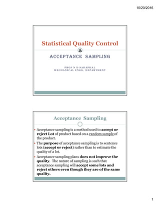
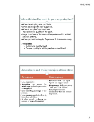
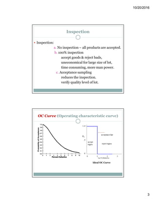
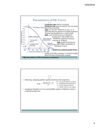
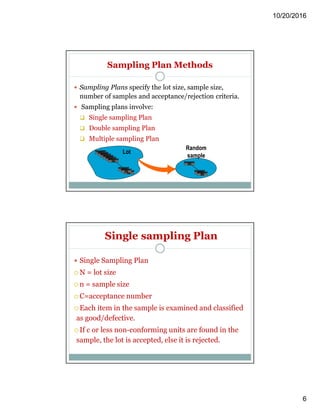
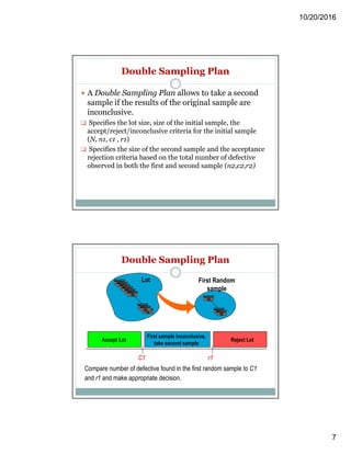
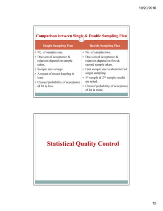
Acceptance sampling is a statistical method used to accept or reject product lots based on random sampling, primarily aimed at evaluating the quality level rather than improving it. Various sampling plans—single, double, and multiple—are employed depending on the situation, each with its advantages and disadvantages, including costs and risks of rejecting good lots or accepting bad ones. The document also discusses statistical quality control concepts, variations, and the use of control charts to monitor and improve processes.

1. ACCEPTANCE SAMPLING
(SQC)
By
Prof N D Sadaphal
Assistant Professor
Sanjivani College of Engineering,
Kopargaon (Maharashtra State) 423601
Mechanical Engineering

2. 10/20/2016
1
ACCEPTANCE SAMPLING
PR OF N D SADA PHAL
MECHA NICAL EN GG. DEPAR TMENT
Statistical Quality Control
&
Acceptance Sampling
 Acceptance sampling is a method used to accept or
reject Lot of product based on a random sample of
the product.
 The purpose of acceptance sampling is to sentence
lots (accept or reject) rather than to estimate the
quality of a lot.
 Acceptance sampling plans does not improve the
quality. The nature of sampling is such that
acceptance sampling will accept some lots and
reject others even though they are of the same
quality.

3. 10/20/2016
2
When this tool be used in your organization?
•When developing new products.
•When dealing with new suppliers.
•When a supplier’s product has
had excellent quality in the past.
•Large numbers of items must be processed in a short
amount of time.
•When product testing is, Expensive & time consuming
Purposes
• Determine quality level.
• Ensure quality is within predetermined level.
AdvantagesAdvantages DisadvantagesDisadvantages
 Less expensive
 Rejection on entire lot
motivates quality improvement
for suppliers
 less handling damage of the
product
 Less man power is involved in
inspection activities.
 It often greatly reduces the
amount of inspection error
 Producer risk - can reject
“good” lots (Type I Error)
 Consumers Risk- can accept
“bad” lots.(Type II Error)
 Sample provides less
information than 100-percent
inspection.
Advantages and Disadvantages of Sampling

4. 10/20/2016
3
Inspection
 Inspection:
a. No inspection – all products are accepted.
b. 100% inspection
accept goods & reject bads,
uneconomical for large size of lot,
time consuming, more man power.
c. Acceptance sampling
reduces the inspection.
verify quality level of lot.
OC Curve (Operating characteristic curve)
Ideal OC Curve

5. 10/20/2016
4
Parameters of OC Curve
Consumer risk- bad lot is accepted.
Producer risk- good lot rejected. This risk should
kept as low as possible.
AQL- It is the max. %defective or max. no. of
defect/hundred for purpose of sampling inspection.
Producer risk should be less or equal to AQL.
RQL- Level of defectiveness so rejected by
sampling plan. AQL & RQL level
decided by negotiation between
customer & producer.
IQL- quality level between
AQL & RQL. Probability of
acceptance is 50%.
AOQL(Avg. outgoing quality limit)-
quality of lot after acceptance. It is lowest quality
level of lot that will generally accepted.
RQL also called as LTPD- lot tolerance % defective
 AOQ (Avg. outgoing quality)- quality that leaves the inspection.
Pd = true percent defective of the lot
Pa = probability of accepting the lot
N = number of items in the lot
n = number of items in the sample
 Acceptance Number (c)- it is a permissible number of defective units in
a selected sample size.

6. 10/20/2016
5
Characteristics of OC Curve
 Changing Lot size- larger lot size will have better characteristic as, it
reduce the risk of error. Lot size increases, sample size also increases.
•Changing sample size-
larger the number items in the
sample, more is the possibility of
finding defects.
 Changing acceptance number- acceptance number
increases, probability of acceptance also increases.

7. 10/20/2016
6
Sampling Plan Methods
 Sampling Plans specify the lot size, sample size,
number of samples and acceptance/rejection criteria.
 Sampling plans involve:
 Single sampling Plan
 Double sampling Plan
 Multiple sampling Plan
Random
sample
Lot
Single sampling Plan
 Single Sampling Plan
 N = lot size
 n = sample size
 C=acceptance number
 Each item in the sample is examined and classified
as good/defective.
 If c or less non-conforming units are found in the
sample, the lot is accepted, else it is rejected.

8. 10/20/2016
7
Double Sampling Plan
 A Double Sampling Plan allows to take a second
sample if the results of the original sample are
inconclusive.
 Specifies the lot size, size of the initial sample, the
accept/reject/inconclusive criteria for the initial sample
(N, n1, c1 , r1)
 Specifies the size of the second sample and the acceptance
rejection criteria based on the total number of defective
observed in both the first and second sample (n2,c2,r2)
Double Sampling Plan
First Random
sample
Lot
C1 r1
First sample inconclusive,
take second sample
Reject LotAccept Lot
Compare number of defective found in the first random sample to C1
and r1 and make appropriate decision.

9. 10/20/2016
8
Double Sampling Plan
C2
Reject LotAccept Lot
Compare the total number of defective in both lots to C2 and make the
appropriate decision
Lot First Random sample
Second Random sample
• A double sampling plan is associated with four
numbers:
• The interpretation of the numbers is shown by an
example:
 1. Inspect a sample of size 20
 2. If the sample contains 3 or less defectives, accept
the lot
 3. If the sample contains more than 5 defectives,
reject the lot.
2121 ccnn and,,
531020 2121  ccnn ,,,Let

10. 10/20/2016
9
 If the sample contains more than 3 and less than or
equal to 5 defectives (i.e., 4 or 5 defectives), then
inspect a second sample of size 10
 5. If the cumulative number of defectives in the
combined sample of 30 is not more than 5, then
accept the lot.
 6. Reject the lot if there are more than 5 defectives
in the combined lot of 30
Multiple sampling Plan
 A Multiple Sampling Plan is similar to the double sampling
plan in that successive trials are made, each of which has
acceptance, rejection and inconclusive options.
Sample Sample
size
Combined samples
size Acceptance
number
Rejection
number
First n1 n1 c1 r1
Second n2 n1+n2 c2 r2
Third n3 n1+n2+n3 c3 r3
Fourth n4 n1+n2+n3+n4 c4 r4
Fifth n5 n1+n2+n3+n4+n5 c5 c5+1

11. 10/20/2016
10
Steps for problem solution
 Step 1 Sample size,
 Step 2 Average Outgoing Quality AOQ,
For double sampling plan:-
 No. of defectives articles= Lot size × percent defective = N × Pd
 No. of non defectives articles= Lot size – no. of defective article=N-(N ×Pd)
 Total no. of defective in first sample, say x=(n × Pd)I
the lot is accepted if, (n × Pd)≤C1, C1=acceptance no. of 1st sample.
For Single sampling plan:-
 For 2nd sample, if no. of defectives >C1 then take 2nd sample for inspection.
if defect ≤ C2 then 2nd lot is accepted. C2=acceptance no. of 2nd sample.
 If defects are greater than C2 lot is rejected.
 No. of defective in 2nd sample say y=(n × Pd)II
 Probability of acceptance for 2nd sample,
lot can be accepted if
Max. defects=C1 (for 1st ) &
Max. defects=(C2-C1) (for 2nd )
 Total probability of acceptance,
 Average Outgoing Quality AOQ,

12. 10/20/2016
11
Table for solving the Problem
0.6 0.7 0.8 0.9 1.0
0 0.549(0.549) 0.819(0.819) 0.499(0.499) 0.406(0.406) 0.368(0.368)
1 0.329(0.878) 0.164(0.983) 0.359(0.808) 0.366(0.772) 0.368(0.736)
2 0.099(0.977) 0.016(0.999) 0.144(0.952) 0.166(0.938) 0.184(0.92)
nP’
c

13. 10/20/2016
12
Single Sampling PlanSingle Sampling Plan Double Sampling PlanDouble Sampling Plan
 No. of samples one.
 Decision of acceptance &
rejection depend on sample
taken.
 Sample size is large.
 Amount of record keeping is
least
 Chance/probability of acceptance
of lot is less.
 No. of samples two.
 Decision of acceptance &
rejection depend on first &
second sample taken.
 First sample size is about half of
single sampling.
 1st sample & 2nd sample results
are noted.
 Chance/probability of acceptance
of lot is more.
Comparison between Single & Double Sampling Plan
Statistical Quality Control

14. 10/20/2016
13
SQC
 It is the collection, analysis & interpretation of
data to solve a particular problem.
 Products of uniform acceptable quality are
manufactured.
Statistical Quality Control
Statistical concept
 Data:- collected for quality control purpose.
Classified as,
 Variables- These are quality characteristics that
are measured. e.g. weight- in KG, diameter in mm.
 Attributes- These are those quality characteristics
that are classified as either present or absent in the
product.
 e.g. Order is either complete or incomplete , Go-No Go
gauge inspection, presence of crack in welding.

15. 10/20/2016
14
Frequency Diagram
 1. Manufacturing variability-
No parts can be produced with identical measurements. Their
will be variation due to manufacturing process or measuring
equipment.
 Histogram
Freq.
Dia. Of pins in mm
join top point of each
histogram rectangle by line, the
obtained graph is known as
frequency polygon.
If we join these points by
smooth curve, obtained graph is
called as frequency distribution.
• Frequency Distribution

16. 10/20/2016
15
Concept of variation
 No two items are exactly alike.
 Some sort of variations in the two items is bound to be
there. In fact it is an integral part of any manufacturing
process.
 This difference in characteristics known as variation.
 This variation may be due to substandard quality of raw
material, carelessness on the part of operator, fault
in machinery system etc.
Types Of Variations
30

17. 10/20/2016
16
Variation due to chance causes
 Variation occurred due to chance.
 This variation is NOT due to defect in machine, Raw
material or any other factors.
 Variation due to slight vibration in machine, sudden
failure of power supply.
 Behave in “random manner”.
 Negligible but Inevitable
 The process is said to be under the state of statistical
control.
31
31
Variation due to Assignable causes
Non – random causes
like:
 Difference in quality of raw material
 Difference in machines
 Difference in operators
 Difference of time
32
32

18. 10/20/2016
17
Graph of sample data plotted over time
Assignable
Cause Variation
Random
Variation
Process
Average 
Control Charts
LCL
UCL
Mean
Mean, Median & Mode
 Mean-
Average of measured reading.
or if frequency of data is given then,
 Median- if set of reading is given
2,9,4,8,10
----median is 8 i.e. central value
2,4,7,8,9,10
-----median is avg. of central two values i.e. 7 & 8 i.e.(7.5)
For calculating median arrange the reading in ascending order.
 Mode- value which occurs more time.
or value having higher position in graph. (last example mode is 1.8)
2,4,8,9,10

19. 10/20/2016
18
Range & Standard Deviation
 Range-
Difference between highest & lowest reading.
Set of readings 2,9,4,8,10
Range= (10-2)=8
 Standard Deviation-
X1, X2,….,Xn are individual reading
is mean
Control charts
 The control chart is a statistical quality control tool used in the monitoring
variation in the characteristics of a product or service
 Data collected from a control chart may form the basis for process improvement.
 UCL = Process Average + 3 Standard Deviations
 LCL = Process Average - 3 Standard Deviations
Process Average
UCL
LCL
X
+ 3
- 3
TIME

20. 10/20/2016
19
X-chart (Variable data)
 It is used to monitor changes in the mean of a process.
 To construct a mean chart we first need to construct the center line
of the chart
 Step 1 calculate mean
 Step 2 calculate Grant mean
 Step 3 standard deviation of the distributed sample means
 Step 4 calculate control limits
 Step 5 plot graph

21. 10/20/2016
20
Control charts for variable
 X-chart & R-chart

22. 10/20/2016
21
 A quality control inspector at the Cocoa Fizz soft drink company
has taken 5 samples with four observations each of the volume of
bottles filled. The data and the computed means are shown in the
table. If the standard deviation of the bottling operation is 0.14
ounces, use this information to develop control limits of three
standard deviations for the bottling operation.