9.0 ~ Lot-by-Lot Acceptance Sampling by Atributes.ppt
1.
KP6373: QUALITY SYSTEMS
Chapter8
Lot-By-Lot Acceptance Sampling by
Attributes & Acceptance Sampling
Systems
1
hjbaba@eng.ukm.my
2.
LEARNING OBJECTIVES
Upon thecompletion of this chapter, the
student is expected:
Know the advantages and disadvantages of sampling;
the types of sampling plans and selection factors;
criteria for formation of lots; criteria for sample
selection; and decisions concerning rejected lots.
Determine the OC curve for single sampling plan.
Determine the equation needed to draw graph of the OC
curve for a double sampling plan.
Know properties of OC curves.
Know the consumer-producer relation of risk, AQL, and
LQ.
2
hjbaba@eng.ukm.my
3.
FUNDAMENTAL CONCEPTS
3
Lot-by-lotacceptance sampling by attributes is the
most common type of sampling.
In lot-by-lot sampling, a predetermined number of
units (sample) from each lot is inspected by attributes.
If the number of “nonconforming” unit is less than
the prescribed minimum, the lot is accepted; if not, the lot
is not accepted (i.e. rejected).
A single sampling plan is defined by the lot size, N,
the sample size, n, and the acceptance number, C.
Example: The plan for, N = 9000, n = 300, C = 2 means
that a lot of 9,000 units has 300 units inspected. If two
or fewer nonconforming units are found in the 300-
unit sample, the lot is accepted. If three or more
nonconforming units are found in the 300-unit sample,
the lot is not accepted (i.e. rejected).
hjbaba@eng.ukm.my
4.
FUNDAMENTAL CONCEPTS…
4
Acceptancesampling can be performed in a
number of situations where there is a consumer -
producer relationship.
5 situations where acceptance sampling of product
will be used:
(1) When the test is destructive (e.g. electrical
fuse), sampling is necessary; otherwise, all
of the product will be destroyed by testing.
(2) When the cost of 100% inspection is high in
relation to the cost of passing a
nonconforming unit.
hjbaba@eng.ukm.my
5.
FUNDAMENTAL CONCEPTS…
5
5situations where acceptance sampling of product
will be used…
(3) When there are many similar units to be
inspected, sampling will produce as good, if not
better results than 100% inspection. This is
true because with manual inspection, fatigue and
boredom cause a higher percentage of
nonconforming product to be passed than
would occur on the average using a sampling
plan.
(4) When the information concerning producer’s
quality, such as and R, p or c charts and Cpk
is not available.
(5) When automated inspection is not available.
X
hjbaba@eng.ukm.my
6.
ADVANTAGES OF ACCEPTANCE
SAMPLINGCOMPARED TO 100%
INSPECTION
6
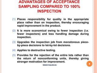
(1) Places responsibility for quality in the appropriate
place rather than on inspection, thereby encouraging
rapid improvement in the product.
(2) It is more economical owing to fewer inspection (i.e.
fewer inspectors) and less handling damage during
inspection.
(3) Upgrades the inspection job from monotonous piece-
by-piece decisions to lot-by-lot decisions.
(4) Applies to destructive testing.
(5) Provides for the rejection of the entire lots rather than
the return of nonconforming units, thereby giving
stronger motivation for improvement.
hjbaba@eng.ukm.my
7.
DISADVANTAGES OF ACCEPTANCE
SAMPLINGCOMPARED TO 100%
INSPECTION
7
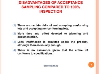
(1) There are certain risks of not accepting conforming
lots and accepting nonconforming lots.
(2) More time and effort devoted to planning and
documentation.
(3) Less information is provided about the product,
although there is usually enough.
(4) There is no assurance given that the entire lot
conforms to specifications.
hjbaba@eng.ukm.my
8.
TYPES OF SAMPLINGPLANS
8
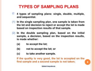
4 types of sampling plans: single, double, multiple,
and sequential.
(1) In the single sampling plan, one sample is taken from
the lot and decision to reject or accept the lot is made
based on inspection results of that sample.
(2) In the double sampling plan, based on the initial
sample, a decision, based on the inspection results,
is made whether:
(a) to accept the lot;
(b) not to accept the lot; or
(c) to take another sample.
If the quality is very good, the lot is accepted on the
first sample and a second sample is not taken;
hjbaba@eng.ukm.my
9.
TYPES OF SAMPLINGPLANS…
9
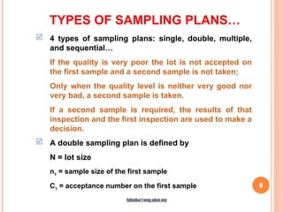
4 types of sampling plans: single, double, multiple,
and sequential…
If the quality is very poor the lot is not accepted on
the first sample and a second sample is not taken;
Only when the quality level is neither very good nor
very bad, a second sample is taken.
If a second sample is required, the results of that
inspection and the first inspection are used to make a
decision.
A double sampling plan is defined by
N = lot size
n1
= sample size of the first sample
C1
= acceptance number on the first sample
hjbaba@eng.ukm.my
10.
TYPES OF SAMPLINGPLANS…
10
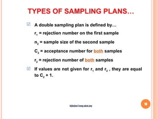
A double sampling plan is defined by…
r1
= rejection number on the first sample
n2
= sample size of the second sample
C2
= acceptance number for both samples
r2
= rejection number of both samples
If values are not given for r1
and r2
, they are equal
to C2
+ 1.
hjbaba@eng.ukm.my
11.
EXAMPLE
11
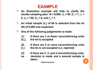
An illustrativeexample will help to clarify the
double sampling plan: N = 9,000, n1
= 60, C1
= 1, r1
=
5, n2
= 150, C2
= 6, and r2
= 7.
An initial sample (n1
) of 60 is selected from the lot
(N) of 9,000 and inspected.
One of the following judgements is made:
(1) If there are 1 or fewer nonconforming units
(C1
), the lot is accepted.
(2) If there are 5 or more nonconforming units
(r1
) the lot is not accepted (i.e. rejected)
(3) If there are 2, 3, and 4 nonconforming units,
no decision is made and a second sample is
taken.
hjbaba@eng.ukm.my
12.
EXAMPLE…
12
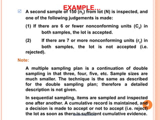
A secondsample of 150 (n2
) from lot (N) is inspected, and
one of the following judgements is made:
(1) If there are 6 or fewer nonconforming units (C2
) in
both samples, the lot is accepted.
(2) If there are 7 or more nonconforming units (r2
) in
both samples, the lot is not accepted (i.e.
rejected).
Note:
A multiple sampling plan is a continuation of double
sampling in that three, four, five, etc. Sample sizes are
much smaller. The technique is the same as described
for the double sampling plan; therefore a detailed
description is not given.
In sequential sampling, items are sampled and inspected
one after another. A cumulative record is maintained, and
a decision is made to accept or not to accept (i.e. reject)
the lot as soon as there is sufficient cumulative evidence.
hjbaba@eng.ukm.my
13.
FORMATION OF LOTS
13
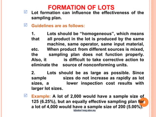
Lot formation can influence the effectiveness of the
sampling plan.
Guidelines are as follows:
1. Lots should be “homogeneous”, which means
that all product in the lot is produced by the same
machine, same operator, same input material,
etc. When product from different sources is mixed,
the sampling plan does not function properly.
Also, it is difficult to take corrective action to
eliminate the source of nonconforming units.
2. Lots should be as large as possible. Since
sample sizes do not increase as rapidly as lot
sizes, a lower inspection cost results with
larger lot sizes.
Example: A lot of 2,000 would have a sample size of
125 (6.25%), but an equally effective sampling plan for
a lot of 4,000 would have a sample size of 200 (5.00%).
hjbaba@eng.ukm.my
14.
SAMPLE SELECTION
14
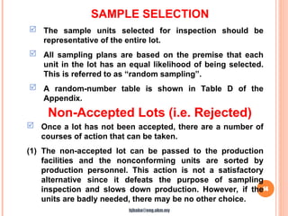
Thesample units selected for inspection should be
representative of the entire lot.
All sampling plans are based on the premise that each
unit in the lot has an equal likelihood of being selected.
This is referred to as “random sampling”.
A random-number table is shown in Table D of the
Appendix.
Non-Accepted Lots (i.e. Rejected)
Once a lot has not been accepted, there are a number of
courses of action that can be taken.
(1) The non-accepted lot can be passed to the production
facilities and the nonconforming units are sorted by
production personnel. This action is not a satisfactory
alternative since it defeats the purpose of sampling
inspection and slows down production. However, if the
units are badly needed, there may be no other choice.
hjbaba@eng.ukm.my
15.
15
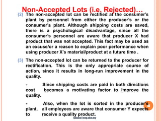
(2) The non-acceptedlot can be rectified at the consumer’s
plant by personnel from either the producer’s or the
consumer’s plant. Although shipping costs are saved,
there is a psychological disadvantage, since all the
consumer’s personnel are aware that producer X had
product that was not accepted. This fact may be used as
an excuse/or a reason to explain poor performance when
using producer X’s material/product at a future time .
(3) The non-accepted lot can be returned to the producer for
rectification. This is the only appropriate course of
action, since it results in long-run improvement in the
quality.
- Since shipping costs are paid in both directions
cost becomes a motivating factor to improve the
quality.
- Also, when the lot is sorted in the producer’s
plant, all employees are aware that consumer Y expects
to receive a quality product.
Non-Accepted Lots (i.e. Rejected)…
hjbaba@eng.ukm.my
16.
16
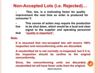
- This, too,is a motivating factor for quality
improvement the next time an order is produced for
consumer Y.
- This course of action may require the production
line to be shut down, which would be a loud and clear
signal to the supplier and operating personnel
that “quality is important”.
Note:
It is assumed that non-accepted lots will receive 100%
inspection and nonconforming units are discarded.
A resubmitted lot is not normally re-inspected, but if it is,
the inspection should be confine to the original
nonconformity.
Since, the nonconforming units are discarded, a
resubmitted lot will have fewer units from the original.
Non-Accepted Lots (i.e. Rejected)…
hjbaba@eng.ukm.my
17.
17
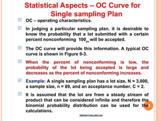
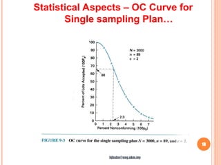
OC –operating characteristics.
In judging a particular sampling plan, it is desirable to
know the probability that a lot submitted with a certain
percent nonconforming 100po
will be accepted.
The OC curve will provide this information. A typical OC
curve is shown in Figure 9-3.
When the percent of nonconforming is low, the
probability of the lot being accepted is large and
decreases as the percent of nonconforming increases.
Example: A single sampling plan has a lot size, N = 3,000,
a sample size, n = 89, and an acceptance number, C = 2.
It is assumed that the lot are from a steady stream of
product that can be considered infinite and therefore the
binomial probability distribution can be used for the
calculations.
Statistical Aspects – OC Curve for
Single sampling Plan
hjbaba@eng.ukm.my
19
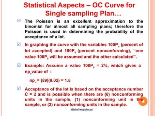
The Poissonis an excellent approximation to the
binomial for almost all sampling plans; therefore the
Poisson is used in determining the probability of the
acceptance of a lot.
In graphing the curve with the variables 100Pa
(percent of
lot accepted) and 100P0
(percent nonconforming), “one
value 100P0
will be assumed and the other calculated”.
Example: Assume a value 100P0
= 2%, which gives a
npo
value of :
npo
= (89)(0.02) = 1.8
Acceptance of the lot is based on the acceptance number
C = 2 and is possible when there are (0) nonconforming
units in the sample, (1) nonconforming unit in the
sample, or (2) nonconforming units in the sample.
Statistical Aspects – OC Curve for
Single sampling Plan…
hjbaba@eng.ukm.my
20.
20
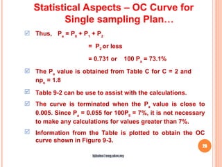
Thus, Pa
=P0
+ P1
+ P2
= P2
or less
= 0.731 or 100 Pa
= 73.1%
The Pa
value is obtained from Table C for C = 2 and
npo
= 1.8
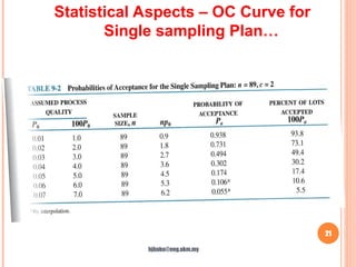
Table 9-2 can be use to assist with the calculations.
The curve is terminated when the Pa
value is close to
0.005. Since Pa
= 0.055 for 100P0
= 7%, it is not necessary
to make any calculations for values greater than 7%.
Information from the Table is plotted to obtain the OC
curve shown in Figure 9-3.
Statistical Aspects – OC Curve for
Single sampling Plan…
hjbaba@eng.ukm.my
22
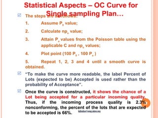
The stepsare as follows:
1. Assume P0
value;
2. Calculate npo
value;
3. Attain Pa
values from the Poisson table using the
applicable C and npo
values;
4. Plot point (100 P0
, 100 Pa
)
5. Repeat 1, 2, 3 and 4 until a smooth curve is
obtained.
“To make the curve more readable, the label Percent of
Lots (expected to be) Accepted is used rather than the
probability of Acceptance”.
Once the curve is constructed, it shows the chance of a
Lot being accepted for a particular incoming quality.
Thus, if the incoming process quality is 2.3%
nonconforming, the percent of the lots that are expected
to be accepted is 66%.
Statistical Aspects – OC Curve for
Single sampling Plan…
hjbaba@eng.ukm.my
23.
23
Similarly, if55 lot from a process that is 2.3%
nonconforming is inspected using this sampling plan,
36 {i.e. [(55)(0.66) = 36]} will be accepted and 19 {i.e.
(55 –36) = 19} will be unacceptable.
This OC curve is unique to the sampling plan defined
by N = 3,000, n = 89 and C = 2.
If this sampling plan does not give the desired
effectiveness, then the sampling plan should be
changed and a new OC curve constructed and
evaluated.
Statistical Aspects – OC Curve for
Single sampling Plan…
hjbaba@eng.ukm.my
24.
24
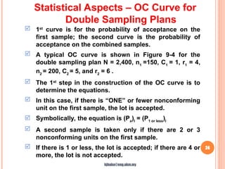
1st
curve isfor the probability of acceptance on the
first sample; the second curve is the probability of
acceptance on the combined samples.
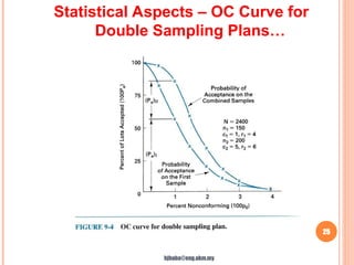
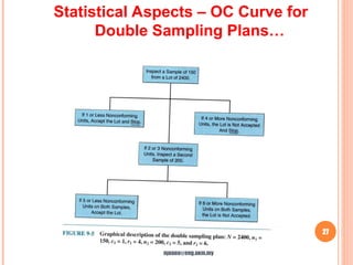
A typical OC curve is shown in Figure 9-4 for the
double sampling plan N = 2,400, n1
=150, C1
= 1, r1
= 4,
n2
= 200, C2
= 5, and r2
= 6 .
The 1st
step in the construction of the OC curve is to
determine the equations.
In this case, if there is “ONE” or fewer nonconforming
unit on the first sample, the lot is accepted.
Symbolically, the equation is (Pa
)I
= (P1 or less
)I
A second sample is taken only if there are 2 or 3
nonconforming units on the first sample.
If there is 1 or less, the lot is accepted; if there are 4 or
more, the lot is not accepted.
Statistical Aspects – OC Curve for
Double Sampling Plans
hjbaba@eng.ukm.my
26
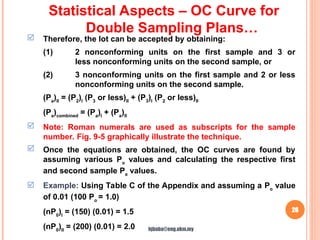
Therefore, thelot can be accepted by obtaining:
(1) 2 nonconforming units on the first sample and 3 or
less nonconforming units on the second sample, or
(2) 3 nonconforming units on the first sample and 2 or less
nonconforming units on the second sample.
(Pa
)II
= (P2
)I
(P3
or less)II
+ (P3
)I
(P2
or less)II
(Pa
)combined
= (Pa
)I
+ (Pa
)II
Note: Roman numerals are used as subscripts for the sample
number. Fig. 9-5 graphically illustrate the technique.
Once the equations are obtained, the OC curves are found by
assuming various Po
values and calculating the respective first
and second sample Pa
values.
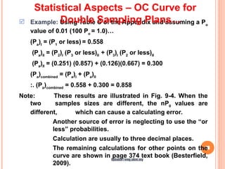
Example: Using Table C of the Appendix and assuming a Po
value
of 0.01 (100 Po
= 1.0)
(nP0
)I
= (150) (0.01) = 1.5
(nP0
)II
= (200) (0.01) = 2.0
Statistical Aspects – OC Curve for
Double Sampling Plans…
hjbaba@eng.ukm.my
28
Example: UsingTable C of the Appendix and assuming a Po
value of 0.01 (100 Po
= 1.0)…
(Pa
)I
= (P1
or less) = 0.558
(Pa
)II
= (P2
)I
(P3
or less)II
+ (P3
)I
(P2
or less)II
(Pa
)II
= (0.251) (0.857) + (0.126)(0.667) = 0.300
(Pa
)combined
= (Pa
)I
+ (Pa
)II
:. (Pa
)combined
= 0.558 + 0.300 = 0.858
Note: These results are illustrated in Fig. 9-4. When the
two samples sizes are different, the nP0
values are
different, which can cause a calculating error.
Another source of error is neglecting to use the “or
less” probabilities.
Calculation are usually to three decimal places.
The remaining calculations for other points on the
curve are shown in page 374 text book (Besterfield,
2009).
Statistical Aspects – OC Curve for
Double Sampling Plans…
hjbaba@eng.ukm.my
29.
29
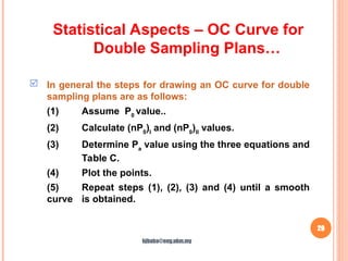
In generalthe steps for drawing an OC curve for double
sampling plans are as follows:
(1) Assume P0
value..
(2) Calculate (nP0
)I
and (nP0
)II
values.
(3) Determine Pa
value using the three equations and
Table C.
(4) Plot the points.
(5) Repeat steps (1), (2), (3) and (4) until a smooth
curve is obtained.
Statistical Aspects – OC Curve for
Double Sampling Plans…
hjbaba@eng.ukm.my
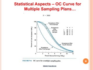
30.
30
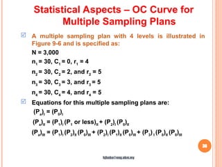
A multiplesampling plan with 4 levels is illustrated in
Figure 9-6 and is specified as:
N = 3,000
n1
= 30, C1
= 0, r1
= 4
n2
= 30, C2
= 2, and r2
= 5
n3
= 30, C3
= 3, and r3
= 5
n4
= 30, C4
= 4, and r4
= 5
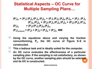
Equations for this multiple sampling plans are:
(Pa
)I
= (P0
)I
(Pa
)II
= (P1
)I
(P1
or less)II
+ (P2
)I
(P0
)II
(Pa
)III
= (P1
)I
(P2
)II
(P0
)III
+ (P2
)I
(P1
)II
(P0
)III
+ (P3
) I
(P0
)II
(P0
)III
Statistical Aspects – OC Curve for
Multiple Sampling Plans
hjbaba@eng.ukm.my
32
(Pa
)IV
= (P1
)I
(P2
)II
(P1
)III
(P0
)IV
+ (P1
)I
(P3
)II
(P0
)III
(P0
)IV
+(P2
) I
(P1
)II
(P1
)III
(P0
)IV
+ (P2
)I
(P2
)II
(P0
)III
(P0
)IV
+ (P3
)I
(P0
)II
(P1
)III
(P0
)IV
+ (P3
)I
(P1
)II
(P0
)III
(P0
)IV
(Pa
)combined
= (Pa
)I
+ (Pa
)II
+ (Pa
)III
+ (Pa
)IV
###
Using the equations above and varying the fraction
nonconforming, P0
, the OC curve of Figure 9–6 is
constructed.
This a tedious task and is ideally suited for the computer.
An OC curve evaluates the effectiveness of a particular
sampling plan. If the sampling is not satisfactory, as shown
by the OC curve, another sampling plan should be selected
and its OC is constructed.
Statistical Aspects – OC Curve for
Multiple Sampling Plans…
hjbaba@eng.ukm.my
33.
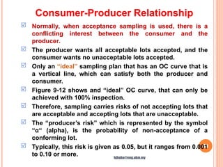
33
Normally, whenacceptance sampling is used, there is a
conflicting interest between the consumer and the
producer.
The producer wants all acceptable lots accepted, and the
consumer wants no unacceptable lots accepted.
Only an “ideal” sampling plan that has an OC curve that is
a vertical line, which can satisfy both the producer and
consumer.
Figure 9-12 shows and “ideal” OC curve, that can only be
achieved with 100% inspection.
Therefore, sampling carries risks of not accepting lots that
are acceptable and accepting lots that are unacceptable.
The “producer’s risk” which is represented by the symbol
“α“ (alpha), is the probability of non-acceptance of a
conforming lot.
Typically, this risk is given as 0.05, but it ranges from 0.001
to 0.10 or more.
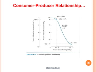
Consumer-Producer Relationship
hjbaba@eng.ukm.my
35
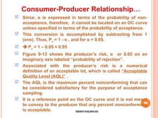
Since, αis expressed in terms of the probability of non-
acceptance, therefore, it cannot be located on an OC curve
unless specified in terms of the probability of acceptance.
This conversion is accomplished by subtracting from 1
(one). Thus, Pa
= 1 - α , and for α = 0.05,
Pa
= 1 – 0.05 = 0.95
Figure 9-13 shows the producer’s risk, α or 0.05 on an
imaginary axis labeled “probability of rejection”.
Associated with the producer’s risk is a numerical
definition of an acceptable lot, which is called “Acceptable
Quality Level (AQL)” .
The AQL is the maximum percent nonconforming that can
be considered satisfactory for the purpose of acceptance
sampling.
It is a reference point on the OC curve and it is not meant
to convey to the producer that any percent nonconforming
is acceptable.
Consumer-Producer Relationship…
hjbaba@eng.ukm.my
37
The onlyway the producer can be guaranteed that a lot
will be accepted is to have 0% nonconforming or to have
the number of nonconforming in the lot less than or
equal to the acceptance number.
Summary: The producer’s quality goal is to meet or
exceed the specifications so that no nonconforming
units are present in the lot.
Example: For the sampling plan, N = 4,000, n = 300, and
C = 4, the AQL = 0.7% for 100α = 5% as shown in Figure
9-13.
In other words, product that is 0.7% nonconforming will
have a non-acceptance probability of 0.05 or 5%.
The “consumer’s risk”, represented by the symbol β
(beta), is the probability of acceptance of a
nonconforming lot. This risk is frequently given as 0.10
or 10%.
Consumer-Producer Relationship…
hjbaba@eng.ukm.my
38.
38
Since, βis expressed in terms of probability of
acceptance, therefore, no conversion is necessary.
Associated with the consumer’s risk is a numerical
definition of a nonconforming lot, called “Limiting Quality
(LQ)”.
The LQ is the percent nonconforming in a lot or batch for
which, for acceptance sampling purposes, the consumer
wishes the probability of acceptance to be low.
For the sampling plan in Figure 9-13, the LQ = 2.6% for
100β = 10%. In other words, lots that are 2.6%
nonconforming will have a 10% chance of being accepted.
A better understanding of the concept of acceptance
sampling can be obtained from an example.
Suppose that over a period of time, 15 lots of 3,000 each
are shipped by the producer to the consumer. The lots are
2% nonconforming and a sampling plan of n = 89 and C =
2 is used to determine acceptance.
Consumer-Producer Relationship…
hjbaba@eng.ukm.my
39.
39
Figure 9-15shows this information by a solid line.
The OC curve for this sampling plan (Refer to Figure 9-3)
shows that the percent of lots accepted for a 2%
nonconforming lot is 73.1%.
Thus, 11 lots (15 X 0.731 = 10.97) are accepted by the
consumer, as shown by the “wavy line”.
Four lots are not accepted by the sampling plan and
returned to the producer for rectification, as shown by the
“dashed line”.
These 4 lots receive 100% inspection and are returned to
the consumer with 0% nonconforming, as shown by a
“dashed line”.
A summary of what the consumer actually receives is
shown at the bottom of Figure 9-15.
Consumer-Producer Relationship…
hjbaba@eng.ukm.my
41
2% or240, of the rectified lots are discarded by the
producer, which gives 11,760 rather than 12,000.
The calculation shows that the consumer actually
receives 1.47% nonconforming, whereas the producer’s
quality is 2% nonconforming.
Note: It should be emphasized that the acceptance
sampling system works only when non-accepted lots are
returned to the producer and rectified.
The AQL for this particular sampling plan at α = 0.05 is
0.9%; therefore, the producer at 2% nonconforming is
not achieving the desired quality level.
Consumer-Producer Relationship…
hjbaba@eng.ukm.my
42.
42
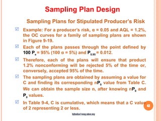
Sampling Plans forStipulated Producer’s Risk
Sampling Plan Design
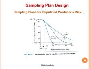
Example: For a producer’s risk, α = 0.05 and AQL = 1.2%,
the OC curves for a family of sampling plans are shown
in Figure 9-19.
Each of the plans passes through the point defined by
100 Pa
= 95% (100 α = 5%) and P0.95
= 0.012.
Therefore, each of the plans will ensure that product
1.2% nonconforming will be rejected 5% of the time or,
conversely, accepted 95% of the time.
The sampling plans are obtained by assuming a value for
C and finding its corresponding nP0
value from Table C.
We can obtain the sample size n, after knowing nP0
and
P0
values.
In Table 9-4, C is cumulative, which means that a C value
of 2 representing 2 or less.
hjbaba@eng.ukm.my
43.
43
Sampling Plans forStipulated Producer’s Risk…
Sampling Plan Design
hjbaba@eng.ukm.my
44.
44
Sampling Plans forStipulated Producer’s Risk…
Sampling Plan Design
hjbaba@eng.ukm.my
45.
45
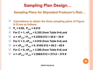
Sampling Plans forStipulated Producer’s Risk…
Sampling Plan Design…
Calculations to obtain the three sampling plans of Figure
9-19 are as follows:
Pa
= 0.95; P0.95
= 0.012
For C = 1, nP0.95
= 0.355 (from Table 9-4) and
n = nP0.95
/ P0.95
= 0.355/0.012 = 29.6 ~ 30 #
For C = 2, nP0.95
= 0.818 (from Table 9-4) and
n = nP0.95
/ P0.95
= 0. 818/0.012 = 68.2 ~ 68 #
For C = 6, nP0.95
= 3.286 (from Table 9-4) and
n = nP0.95
/ P0.95
= 3.286/0.012 = 273.9 ~ 274 #
hjbaba@eng.ukm.my
46.
46
Sampling Plans forStipulated Consumer’s Risk…
Sampling Plan Design…
Example: For a consumer’s risk, β = 0.10 and LQ =
6.02% (LQ – Limiting Quality), the OC curves for a
family of sampling plans are shown in Figure 9-20.
Each of the plans passes through the point defined by
Pa
= 0.10 (β = 0.10) and P0.10
= 0.060.
Therefore, each of the plans will ensure that product
6.0% nonconforming will be accepted 10% of the time.
The sampling plans are determined in the same
manner as used for a stipulated producer’s risk .
hjbaba@eng.ukm.my
47.
47
Sampling Plans forStipulated Consumer’s Risk…
Sampling Plan Design…
hjbaba@eng.ukm.my
48.
48
Sampling Plans forStipulated Consumer’s Risk…
Sampling Plan Design…
Calculations to obtain the three sampling plans of Figure
9-20 are as follows:
Pa
= 0.10; P0.10
= 0.060
For C = 1, nP0.10
= 3.890 (from Table 9-4) and
n = nP0.10
/ P0.10
= 3.890/0.060 = 64.8 => 65 #
For C = 3, nP0.10
= 6.681 (from Table 9-4) and
n = nP0.10
/ P0.10
= 6.681 /0.060 = 111.4 => 111 #
For C = 7, nP0.10
= 11.771 (from Table 9-4) and
n = nP0.10
/ P0.10
= 11.771 /0.060 = 196.2 =>196 #
hjbaba@eng.ukm.my
49.
49
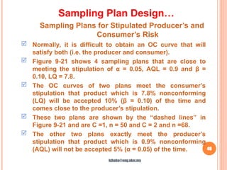
Sampling Plans forStipulated Producer’s and
Consumer’s Risk
Sampling Plan Design…
Normally, it is difficult to obtain an OC curve that will
satisfy both (i.e. the producer and consumer).
Figure 9-21 shows 4 sampling plans that are close to
meeting the stipulation of α = 0.05, AQL = 0.9 and β =
0.10, LQ = 7.8.
The OC curves of two plans meet the consumer’s
stipulation that product which is 7.8% nonconforming
(LQ) will be accepted 10% (β = 0.10) of the time and
comes close to the producer’s stipulation.
These two plans are shown by the “dashed lines” in
Figure 9-21 and are C =1, n = 50 and C = 2 and n =68.
The other two plans exactly meet the producer’s
stipulation that product which is 0.9% nonconforming
(AQL) will not be accepted 5% (α = 0.05) of the time.
hjbaba@eng.ukm.my
50.
50
Sampling Plans forStipulated Producer’s and
Consumer’s Risk…
Sampling Plan Design…
hjbaba@eng.ukm.my
51.
51
Sampling Plans forStipulated Producer’s and
Consumer’s Risk…
Sampling Plan Design…
These two plans are shown by the solid lines and are C =
1, n = 39 and C = 2, n = 91 (Figure 9-21).
In order to determine the plans, the first step is to find the
ratio of P0.10
/ P0.95
,which is
P0.10
/ P0.95
= 0.078/0.009 = 8.667 #
From the ratio column of Table 8-4, the ratio of 8.667 falls
between the row for C = 1 and the row for C = 2.
Thus, plans that exactly meet the consumer’s stipulation
of LQ = 7.8% for β = 0.10.
The calculations are shown in pg. 394 and 396 of the text
book (Besterfield, 2009).
hjbaba@eng.ukm.my


![23
Similarly, if 55 lot from a process that is 2.3%
nonconforming is inspected using this sampling plan,
36 {i.e. [(55)(0.66) = 36]} will be accepted and 19 {i.e.
(55 –36) = 19} will be unacceptable.
This OC curve is unique to the sampling plan defined
by N = 3,000, n = 89 and C = 2.
If this sampling plan does not give the desired
effectiveness, then the sampling plan should be
changed and a new OC curve constructed and
evaluated.
Statistical Aspects – OC Curve for
Single sampling Plan…
hjbaba@eng.ukm.my](https://image.slidesharecdn.com/9-260201142934-16346fb4/85/9-0-Lot-by-Lot-Acceptance-Sampling-by-Atributes-ppt-23-320.jpg)


![AcceptanceSampling for students uni[1].ppt](https://cdn.slidesharecdn.com/ss_thumbnails/acceptancesampling1-250204230443-7d8ea06b-thumbnail.jpg?width=640&height=640&fit=bounds)


