1. 1 | P a g e
Using Simulation to Compare and Evaluate Single & Double Sampling Plans
Asmar Farooq
Abstract. Using simulation as the main tool, operating characteristic curves are generated for
single and double sampling plan in order to analyze and select the optimum sampling plan.
Single Sampling plan turns out to be both simple and yields better quality lots, while double
sampling plan is found to be more useful when cost of sampling or timing is a constraint.
Keywords. Acceptance sampling, hyper geometric distribution, Operating Characteristic curve,
probability of acceptance, Type I and II errors, Average Outgoing Quality, Average Sampling
Number
2. 2 | P a g e
Introduction. Acceptance sampling is a statistical method that is applied on a batch of
production items to determine whether to accept or reject the lot. It is part of the quality control
process to ensure that the incoming items being received from the supplier satisfies
predetermined standards. Before the acceptance sampling procedure can begin, the criteria to
accept and reject the lot are clearly defined, and cannot be changed once the procedure begins. A
sample of size ‘n’ is randomly selected from the lot size ‘N’ and is tested for acceptance based
on the predefined criteria. If the lot is rejected, it may be subject to 100% inspection or it can be
returned back to the supplier for credit or replacement.
Acceptance sampling method is mainly useful under one or more of the following
conditions:
1. The time required to inspect all items in the lot is either not available or is too costly.
2. The process of testing negatively affects the unit’s lifetime or if testing is destructive to the
very item being tested.
3. The cost or time consequences of passing some percent of defective items is relatively lower
and/or manageable.
4. Testing large number of items can cause fatigue or boredom which can lead to unexpected
inspection errors.
It must be noted that the consequence of not testing the entire batch will lead to some likelihood
or risk in making wrong inference about the quality of the lot. These are termed as producer’s
and consumer’s risks.
Producer’s Risk. This is also known as Type I error and is denoted by α. It is the probability of
rejecting a lot given that the lot is good. In other words, it is risk that the supplier takes in that a
shipment with less than (1- α)% quality will be rejected. α is commonly set at 5.0%.
Consumer’s Risk. This is also known as Type II error and denoted by β. It is the probability of
accepting a lot given that the lot is bad. In other words, it is risk that the consumer takes in that a
shipment with more than (1- β)% quality will be accepted. β is commonly set at 10.0%.
3. 3 | P a g e
Types of sampling plans.
1. Single sampling plan. This is the most common and easiest plan to use. It follows the
flowchart below.
Figure 1
2. Double sampling plan. The procedure in this plan is very similar to the single sampling plan
except in case of an event d > b (Step 3), second random sample of size ‘n’ is selected and tested.
If d1 + d2 ≤ c, then the sample is accepted, otherwise rejected. ‘c’ is defined as the total number
of defective items allowed in a total of two random samples.
3. Multiple sampling plan. Multiple sampling plan is an extension of double sampling plan
where instead of two, more than two samples are allowed to be inspected from the same lot, if
the prior samples have failed the inspection test.
Simulation can be a great tool in determining the sampling plan that will give the optimal results
for any given event. One such arbitrary event is examined in this paper, and both the single and
double sampling plans are used and later analyzed for optimum plan selection.
No
Yes
STEP1: Randomly select
a sample of n from N
STEP 2: Inspect all items in
sample n for defects
STEP 3:
d ≤ b ?
Reject Lot
N = number of items in a lot
n = number of items selected as a
sample from the lot.
d = total number of defective items
found in a sample ‘n’ after inspection
b =total number of defectives items
allowed in a sample for acceptance.
Accept lot
4. 4 | P a g e
Hypergeometric Distribution. Before we can begin the simulation of sampling plans, it is
necessary to introduce Hypergeometric distribution. It is a discrete probability distribution that
describes the probability of ‘d’ success in ‘n’ draw outs without replacement from a finite
population of size ‘N’ containing exactly ‘D’ successes. Hypergeometric distribution is closely
linked with sampling plans as it is demonstrate below. Success, in this case, translates to a
defective item.
𝑃(𝑋) =
( 𝐷
𝑑)( 𝑁−𝐷
𝑛−𝑑)
( 𝑁
𝑛)
where: n = sample size N = lot size
d = number of defective items in a sample D = total defective items present in a lot
then P(d) is the probability of finding ‘d’ defective items in the sample.
For example, from a lot of 100 items with 10 defective items, a sample of 20 is items is taken,
then the probability that there are no defective items in a sample is P(d=0)
Analytically, 𝑃(𝑑 = 0) =
(10
0 )(100−10
20−0 )
(100
20 )
= 00.09511 or about 9.5%
Using simulation we get the same result. Please note that defective items are represented by 1.
set.seed(123) #Set seed at 123
m=10^6; n=20; d =numeric(m);
N =sample(c((numeric(90)),rep(1,10)),100) #Generates a random sample of
ninety 0’s and ten 1s.
for(i in 1:m)
{
x = sample(N,n) # Using loop, a sample of n is taken
d[i]=sum(x) from N, and total # of defective
} items are stored in vector d
mean(d==0); # Probability of 0 defective items.
0.094814
cutp=(0:(max(d)+1))-.5;
hist(d,breaks=cutp,prob=T, xlab="# of defects", ylab="Probability",
main="Histogram");
lines(0:10,dhyper(0:10,10,90,20),col="blue"); #overlays the analytically
derived curve on top of the
simulated histogram
5. 5 | P a g e
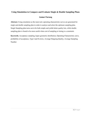
Figure 2 demonstrates that the simulation can provide very close approximation to actual
probabilities. The blue curve is generated using the Hypergeometric distribution function.
Figure 2
Operating Characteristic Curve. The operating characteristic or OC curve is an important tool
which can help discriminate between the quality of the items in a lot being received with the
probability of its acceptance. The curve shows the probability that a given sampling plan will
result in lots with various fractions defective being accepted.
Analytically, we can compute the OC curve using Hypergeometric distribution function for any
given ‘N’, ‘n’ and ‘b’, however, it becomes difficult and complicated for double and multiple
sampling plans. Using simulation, it will be shown that simulation can be a quick and useful tool
to create OC curve chart.
An arbitrary situation is created where a QC Manager is seeking to determine a sampling plan
based on the OC curves for single and double sampling plan. Let the lot size ‘N’ be 500 units and
the sample size ‘n’ be 30. If a sample of 30 gets more than b=4 defective item, then the lot is
rejected, otherwise it is accepted. With these conditions, the event is simulated.
6. 6 | P a g e
Single Sampling plan simulation
set.seed(100) #Setting seed at 100
m = 10^5; N=500; n=30; b=4; #Input the constants
accept=numeric(m); #Stores information whether the lot is
accepted or rejected. (1=accept, 0= reject)
prop = seq(from=0, to=0.4, by=0.01); #Creates a sequence of proportion defective
item in a lot for which probability of
acceptance is generated.
prob.accept = numeric(length(prop));
for(j in 1:length(prop)) #The function of this loop is to find
acceptance probability for each value of
{ defective proportion
for(i in 1:m)
{ s=sample((rbinom(N,1,prop[j])),n) #Here a sample of n is generated out of a lot
N using binomial distribution function for
each defective proportion.
if((sum(s))<=b) { accept[i]=1} else {accept[i]=0} #Using the if statement, we
separate the accepted and rejected
} lot by assigning 0 and 1 values.
prob.accept[j] = mean(accept); } #This is probability of acceptance
plot(prop,prob.accept, type="l"); #Plot of OC Curve
abline(v=c(0,0.025,.05,.075,.1,.15,.2), col="grey");
abline(h=c(0.1,0.2,0.4,0.6,0.8,.85,.9,.95,.99), col="grey");
As mentioned earlier, the study of OC curve is useful tool for analysis of any sampling plan.
Using the code above, OC curve is generated and few points from the graph are given in the
table below.
Proportion defect 0.03 0.07 0.08 0.09 0.1 0.15 0.2 0.25 0.32
# of defect per lot 15 35 40 45 50 75 100 125 160
Acceptance probability 0.998 0.946 0.912 0.872 0.825 0.53 0.25 0.098 0.017
If the lot quality is 0.25 fractions defective, then the probability of acceptance is 10%
(Consumer’s Risk), on the other hand, if the lot quality is 0.07 fractions defective, then the
probability of acceptance is 95% (Producer’s risk).
7. 7 | P a g e
Figure 3 (left) & 4 (right)
Average Outgoing Quality (AOQ). In many sampling plans, if the lot is rejected, then the
entire lot is inspected and all defective items are replaced with the good ones. As the number of
defective items increases in the lot, it becomes more likely for it to be rejected and thus go
through the 100% inspection process. By using this replacement technique, the average outgoing
quality improves in terms of the percent defective. The equation for AOQ =
(𝑃𝑎)(𝑃𝑑)(𝑁−𝑛)
𝑁
where Pa = probability of acceptance and Pd = Proportion defect or (D/N). Using this formula,
AOQ curve easily be generated. The maximum AOQ value is known as Average Outgoing
Quality Limit (AOQL) which is the highest defective percent expected to be present in a lot. The
AOQL in example above comes out to be 0.08.
Multiple Sampling plan simulation. Now, let’s run a different scenario where multiple
sampling plan is implemented. From a lot of N=500, instead of 30, 15 samples (S1) are tested,
half the amount from the single sampling plan. If the first sample has less than or equal to 2
defective items, then the lot is accepted, otherwise, second sample (S2) is taken from the
0.12
1-α
β
8. 8 | P a g e
remaining lot. If the total sum of defective items from samples S1 and S2 exceeds 4, then the lot
is reject, otherwise accepted.
set.seed(100)
m = 10^5; N=500; n=15; b=2; c=4; # c is set at 4 and will be used when the
accept=numeric(m); second sample is taken
prop = seq(from=0, to=0.4, by=0.01);
prob.accept = numeric(length(prop));
count1.p=count2.p=numeric(length(prop)); # Counters are used to count the number of
time second sample is chosen as well as
number of time a lot is chosen given the
for(j in 1:length(prop)) second sample after the second sample is
taken. It is recorded for each defective prop.
{
count1=count2=0 # Counter used for each loop of prop. Their
for(i in 1:m) sum after the end of each loop is recorded in
{ vectors count1.p and count2.p.
lot=rbinom(N,1,prop[j]);
s1=sample(lot,n)
if((sum(s1))<=b) { accept[i]=1} else {
count1 = count1 + 1 #Counter for when the second sample is taken.
lot_count = c(N-sum(lot>0),sum(lot>0))
s1_count = c(n-sum(s1>0),sum(s1>0))
lot_after= lot_count - s1_count;
s2 = sample(c(rep(0,lot_after[1]), rep(1,lot_after[2])), n);
if((sum(s1+s2))<=c) { accept[i]=1; count2=count2+1} else {accept[i]=0}
}
}
prob.accept[j] = mean(accept);
count1.p[j] = sum(count1);
count2.p[j] = sum(count2);
}
plot(prop,prob.accept, type="l");
abline(v=c(0,0.025,.05,.075,.1,.15,.2), col="grey");
abline(h=c(0.1,0.2,0.4,0.6,0.8,.85,.9,.95,.99), col="grey");
plot(prop,count1.p/m, type="l") # Graphs of fraction of times second
abline(v=c(0,.1,.2,.3,.4), col="grey"); sample is accepted as well as the ratio
abline(h=c(0,.2,.4,.6,.8,1), col="grey"); between #of times samples is accepted
par(new=TRUE) to the number of times when the second
plot(prop,count2.p/count1.p, type="l") sample is chosen for inspection
#This code separates the first sample from the
lot, so the second sample can be taken. First, #
of defective and non-defective items are
computed for the lot and sample. The second
sample is taken from the difference of the two.
# The second counter is used when the lot is
accepted after the second sample is taken.
9. 9 | P a g e
Figure 5 (left) & 6 (right)
Proportion defect 0.03 0.07 0.08 0.09 0.1 0.15 0.2 0.25 0.32
# of defect per lot 15 35 40 45 50 75 100 125 160
Pa for single sampling 1.00 0.95 0.91 0.87 0.83 0.53 0.25 0.10 0.02
Pa for double sampling 1.00 0.97 0.95 0.92 0.89 0.68 0.45 0.26 0.10
Comparison. At 95% acceptance probability, the fraction defect is 0.08, which is slightly higher
than the Single sampling plan, but at 10% (consumer’s risk) the fraction defect is 0.32
(significantly higher than the single sampling plan which is 0.25). Furthermore, AOQL is also
higher by 2%.
If both plans are to be judged by their fraction defective rate at Type I and II errors as well as
AOQL values alone, then single sampling plan is certainly better. However, if inspection
requires items to be destroyed or sampling time is an issue, then sampling plan which requires
smaller sampling size is obviously better.
The sample size in single sampling plan always remains constant which in the given example is
30 units. However, in our example of double sampling plan, the first sample size is only 15, and
second sample is only required if the first sample fails to pass. Let’s find out how many times the
AOQL = 0.10 for Double sampling
plan
10. 10 | P a g e
second sample was taken, and what fraction of that sample resulted in acceptance of the lot.
Using the counter vector in the program code, following curves are plotted on the same graph.
Figure 7
sample size is a priority, then double sampling is certainly a better option.
The green curve represents
the probability of accepting
the lot during the first try.
The red curve represents the
probability of selecting the
second sample.
The blue curve represents the
conditional probability of
accepting the lot given that
the first try failed the
inspection test.
Figure 7 shows that at a
reasonable defect level of say
10% or 20%, the probability
of taking another sample is
20% and 60% respectively. It
turns out that if minimizing
Average Sample Number. It is the
average sample size required to make the
decision on acceptance at any given
defect level. It can be easily calculated by
the following formula.
ASN = n1+n2(1-Pa1) where
n1& n2 are 1st
and 2nd
sample size and Pa1
is the probability of accepting the lot after
the first trial.
In Figure 8, on average, only 18 samples
are required to accept the lot if the
defective rate is 10%.
Figure 8
11. 11 | P a g e
Summary and conclusion: The simulation approach to analyze a sampling plan is found to be
very successful with faster results than the analytical approach. Once the program code is
written, any number of events can easily be simulated by just changing the initial constants. In
the example used in this paper, it was found that single sampling plan is a better option when
quality is of utmost importance. The quality can be improved by increasing the sample size or by
choosing a more conservative value of ‘b’. On the other hand, if the inspection requires the
sample items to be destroyed or not enough time is available, then double sampling plan is a
better approach. The simulations method can also be easily extended to multiple sampling plan
with few adjustments.
In order to make the final decision between the two plans, one has to decide whether the average
sampling savings gained by the double sampling plan justifies the additional complexity and
increase in uncertainty in the quality of the lot. The judgment should be made on case by case
basis with factors such as available labor, time, cost and complexity in mind.
12. 12 | P a g e
Bibliography
Prins, Jack , Process or Product Monitoring and Control- Section#2 “Test Product for
Acceptability.” http://www.itl.nist.gov/div898/handbook/pmc/section2/pmc2.htm
13. 13 | P a g e
Appendix.
Complete Simulation 1 for Single Sampling plan.
set.seed(100)
m = 10^5; N=500; n=30; b=4;
accept=numeric(m);
prop = seq(from=0, to=0.4, by=0.01);
prob.accept = numeric(length(prop));
for(j in 1:length(prop))
{
for(i in 1:m)
{
s=sample((rbinom(N,1,prop[j])),n)
if((sum(s))<=b) { accept[i]=1} else {accept[i]=0}
}
prob.accept[j] = mean(accept);
}
plot(prop,prob.accept, type="l");
abline(v=c(0,0.025,.05,.075,.1,.15,.2), col="grey");
abline(h=c(0.1,0.2,0.4,0.6,0.8,.85,.9,.95,.99), col="grey");
AOQ = prob.accept*prop*((N-n)/N)
plot(prop,AOQ, type="l", ylab="Average Outgoing Quality", xlab="Incoming
Percent Defective", main="AOQ Curve for Single Sampling Plan")
abline(v=c(.12))
abline(h=max(AOQ))
Complete Simulation 2 for Double Sampling plan.
set.seed(100)
m = 10^5; N=500; n=15; b=2; c=4;
accept=numeric(m);
prop = seq(from=0, to=0.4, by=0.01);
prob.accept = numeric(length(prop));
count1.p=count2.p=numeric(length(prop));
for(j in 1:length(prop))
{
count1=count2=0
for(i in 1:m)
{
lot=rbinom(N,1,prop[j]);
s1=sample(lot,n)
if((sum(s1))<=b) { accept[i]=1} else
{
count1 = count1 + 1