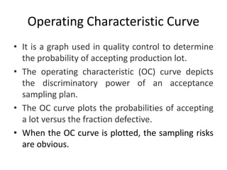
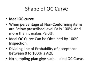
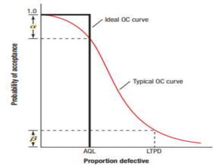
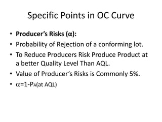
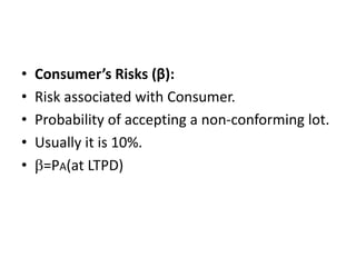
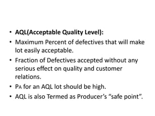
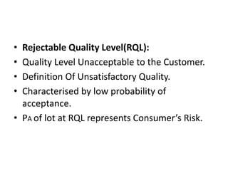
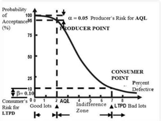
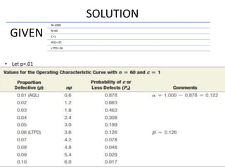
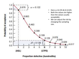
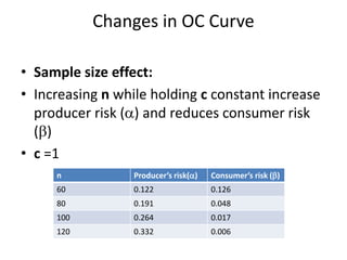
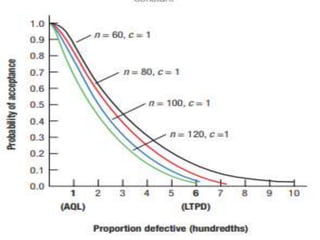
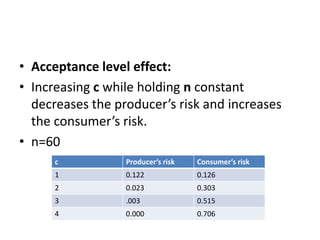
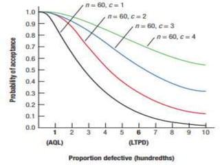
Operating Characteristic Curves
(Advance Sampling Plan)
SANYOGITA
BE+MBA
4th YEAR
CM14226
Operating Characteristic Curve
• It is a graph used in quality control to determine
the probability of accepting production lot.
• The operating characteristic (OC) curve depicts
the discriminatory power of an acceptance
sampling plan.
• The OC curve plots the probabilities of accepting
a lot versus the fraction defective.
• When the OC curve is plotted, the sampling risks
are obvious.
Shape of OC Curve
• Ideal OC curve
• When percentage of Non-Conforming items
are Below prescribed level Pa is 100%. And
more than it makes Pa 0%.
• Ideal OC Curve Can be Obtained By 100%
Inspection.
• Dividing line of Probability of acceptance
Between 0 to 100% is AQL
• No sampling plan give such a ideal OC Curve.
• Typical OC Curve:
• This is Curve Roughly “S” Shaped.
• Obtained by joining points between
Probability of acceptance & Percentage non
conforming items.
• Obtained by Performing Sampling Inspection.
Specific Points in OC Curve
• Producer’s Risks (α):
• Probability of Rejection of a conforming lot.
• To Reduce Producers Risk Produce Product at
a better Quality Level Than AQL.
• Value of Producer’s Risks is Commonly 5%.
• =1-PA(at AQL)
• Consumer’s Risks (β):
• Risk associated with Consumer.
• Probability of accepting a non-conforming lot.
• Usually it is 10%.
• =PA(at LTPD)
• AQL(Acceptable Quality Level):
• Maximum Percent of defectives that will make
lot easily acceptable.
• Fraction of Defectives accepted without any
serious effect on quality and customer
relations.
• PA for an AQL lot should be high.
• AQL is also Termed as Producer’s “safe point”.
• Rejectable Quality Level(RQL):
• Quality Level Unacceptable to the Customer.
• Definition Of Unsatisfactory Quality.
• Characterised by low probability of
acceptance.
• PA of lot at RQL represents Consumer’s Risk.
DEFINATION OF VARIABLES
• PA = The probability of acceptance
• p = Proportion defective
• N = Lot size
• n = Sample size
• c= Acceptance Number
• α = Producer’s Risk
• β= Consumer’s Risk
Steps for drawing OC Curve
• Multiply proportion defective(p) with sample
size (n)
• Record the value for Probability of acceptance
,Pa from poisson probability distribution table
• Then plot OC Curve i.e. proportion defective
vs probability of acceptance.
Given
data
Lot size N
sample size n
Acceptance size c
AQL
LTPD
EXAMPLE
QUESTION
• The Noise King Muffler Shop, a high-volume installer of
replacement exhaust muffler systems, just received a
shipment of 1,000 mufflers. The sampling plan for
inspecting these mufflers calls for a sample size and an
acceptance number . The contract with the muffler
manufacturer calls for an AQL of 1 defective muffler
per 100 and an LTPD of 6 defective mufflers per 100.
Calculate the OC curve for this plan, and determine the
producer’s risk and the consumer’s risk for the plan.
SOLUTION
GIVEN
N=1000
N=60
C=1
AQL=.01
LTPD=.06
• Let p=.01
• Here =12.2% & =12.6%
• Both the values are higher
than the values usually
acceptable .
• We can adjust the risk by
changing the sampling
size.
Changes in OC Curve
• Sample size effect:
• Increasing n while holding c constant increase
producer risk () and reduces consumer risk
()
• c =1
n Producer’s risk() Consumer’s risk ()
60 0.122 0.126
80 0.191 0.048
100 0.264 0.017
120 0.332 0.006
• Acceptance level effect:
• Increasing c while holding n constant
decreases the producer’s risk and increases
the consumer’s risk.
• n=60
c Producer’s risk Consumer’s risk
1 0.122 0.126
2 0.023 0.303
3 .003 0.515
4 0.000 0.706
• We should increase the sample size, which
reduces the consumer’s risk, and increase the
acceptance number, which reduces the
producer’s risk .
• A improved combination can be found by trail
and error.
THANK YOU

Operating characteristic curves

  • 1.
    Operating Characteristic Curves (AdvanceSampling Plan) SANYOGITA BE+MBA 4th YEAR CM14226
  • 2.
    Operating Characteristic Curve •It is a graph used in quality control to determine the probability of accepting production lot. • The operating characteristic (OC) curve depicts the discriminatory power of an acceptance sampling plan. • The OC curve plots the probabilities of accepting a lot versus the fraction defective. • When the OC curve is plotted, the sampling risks are obvious.
  • 3.
    Shape of OCCurve • Ideal OC curve • When percentage of Non-Conforming items are Below prescribed level Pa is 100%. And more than it makes Pa 0%. • Ideal OC Curve Can be Obtained By 100% Inspection. • Dividing line of Probability of acceptance Between 0 to 100% is AQL • No sampling plan give such a ideal OC Curve.
  • 4.
    • Typical OCCurve: • This is Curve Roughly “S” Shaped. • Obtained by joining points between Probability of acceptance & Percentage non conforming items. • Obtained by Performing Sampling Inspection.
  • 6.
    Specific Points inOC Curve • Producer’s Risks (α): • Probability of Rejection of a conforming lot. • To Reduce Producers Risk Produce Product at a better Quality Level Than AQL. • Value of Producer’s Risks is Commonly 5%. • =1-PA(at AQL)
  • 7.
    • Consumer’s Risks(β): • Risk associated with Consumer. • Probability of accepting a non-conforming lot. • Usually it is 10%. • =PA(at LTPD)
  • 8.
    • AQL(Acceptable QualityLevel): • Maximum Percent of defectives that will make lot easily acceptable. • Fraction of Defectives accepted without any serious effect on quality and customer relations. • PA for an AQL lot should be high. • AQL is also Termed as Producer’s “safe point”.
  • 9.
    • Rejectable QualityLevel(RQL): • Quality Level Unacceptable to the Customer. • Definition Of Unsatisfactory Quality. • Characterised by low probability of acceptance. • PA of lot at RQL represents Consumer’s Risk.
  • 11.
    DEFINATION OF VARIABLES •PA = The probability of acceptance • p = Proportion defective • N = Lot size • n = Sample size • c= Acceptance Number • α = Producer’s Risk • β= Consumer’s Risk
  • 12.
    Steps for drawingOC Curve • Multiply proportion defective(p) with sample size (n) • Record the value for Probability of acceptance ,Pa from poisson probability distribution table • Then plot OC Curve i.e. proportion defective vs probability of acceptance. Given data Lot size N sample size n Acceptance size c AQL LTPD
  • 13.
    EXAMPLE QUESTION • The NoiseKing Muffler Shop, a high-volume installer of replacement exhaust muffler systems, just received a shipment of 1,000 mufflers. The sampling plan for inspecting these mufflers calls for a sample size and an acceptance number . The contract with the muffler manufacturer calls for an AQL of 1 defective muffler per 100 and an LTPD of 6 defective mufflers per 100. Calculate the OC curve for this plan, and determine the producer’s risk and the consumer’s risk for the plan.
  • 14.
  • 15.
    • Here =12.2%& =12.6% • Both the values are higher than the values usually acceptable . • We can adjust the risk by changing the sampling size.
  • 16.
    Changes in OCCurve • Sample size effect: • Increasing n while holding c constant increase producer risk () and reduces consumer risk () • c =1 n Producer’s risk() Consumer’s risk () 60 0.122 0.126 80 0.191 0.048 100 0.264 0.017 120 0.332 0.006
  • 18.
    • Acceptance leveleffect: • Increasing c while holding n constant decreases the producer’s risk and increases the consumer’s risk. • n=60 c Producer’s risk Consumer’s risk 1 0.122 0.126 2 0.023 0.303 3 .003 0.515 4 0.000 0.706
  • 20.
    • We shouldincrease the sample size, which reduces the consumer’s risk, and increase the acceptance number, which reduces the producer’s risk . • A improved combination can be found by trail and error.
  • 21.

Editor's Notes

  • #4 Pa is probability of acceptance