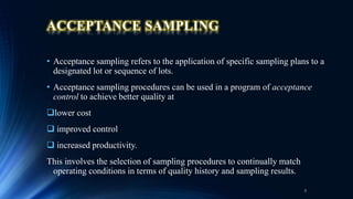
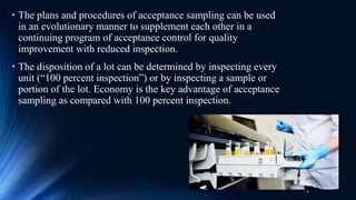
INSPECTION AND TEST
SAMPLING PLAN
PRESENTED BY- SALMAN LATIF
ROLL NO.-27
M. PHARM (QAT)
GUIDE : DR. SONALI MAHAPARALE ,
HOD CHEMISTRY,
DR. D.Y.PATIL COLLGE OF PHARMACY
CONTENTS
♠ ACCEPTANCE SAMPLING
♠ SAMPLING VALIDITY
♠ TYPES OF SAMPLING
♠ TYPES OF DATA
♠ TERMINOLOGY
♠ OPERATING CHARACTERISTIC CURVE
♠ AVERAGE SAMPLE NUMBER CURVE
♠ AVERAGE OUTGOING QUALITY LIMIT
♠ RULE OF THUMB OF SAMPLING
2
ACCEPTANCE SAMPLING
• Acceptance sampling refers to the application of specific sampling plans to a
designated lot or sequence of lots.
• Acceptance sampling procedures can be used in a program of acceptance
control to achieve better quality at
lower cost
 improved control
 increased productivity.
This involves the selection of sampling procedures to continually match
operating conditions in terms of quality history and sampling results.
3
• The plans and procedures of acceptance sampling can be used
in an evolutionary manner to supplement each other in a
continuing program of acceptance control for quality
improvement with reduced inspection.
• The disposition of a lot can be determined by inspecting every
unit (“100 percent inspection”) or by inspecting a sample or
portion of the lot. Economy is the key advantage of acceptance
sampling as compared with 100 percent inspection.
4
ADVANTAGES
1. Economy due to inspecting only part of the product
2. Less handling damage during inspection.
3. Fewer inspectors, thereby simplifying the recruiting and training
problem.
4. Upgrading the inspection job from piece-by-piece decisions to lot-
by-lot decisions.
5. Applicability to destructive testing, with a quantified level of
assurance of lot quality.
6. Rejections of entire lots rather than mere return of the defectives,
thereby providing stronger motivation for improvement.
5
DISADVANTAGES
• 1. There are risks of accepting “bad” lots and of rejecting
“good” lots.
• 2. There is added planning and documentation.
• 3. The sample usually provides less information about the
product than does 100 percent inspection.
6
• Acceptance sampling under a system of acceptance control
provides assurance that lots of product are acceptable for use.
• It is assumed that acceptable product is normally being submitted
by honest , conscientious, capable suppliers.
• The plans provide warnings of discrepancies as a means of
forestalling use of the product while providing signals of the
presence of assignable causes for both the producer and the
consumer.
• If this is not so, other means of dealing with the supplier should
be used—such as discontinuance or 100 percent inspection. This is
why it is called acceptance sampling.
7
Why Is Sampling Valid?
Materials
Finished
Products
LOT LOT LOT
Manufacturing
Process
Samples
From Lot
LOT
8
• The broad scheme of use of sampling is shown in Figure .
• It is universally realized that inspection of a sample gives
information then and there about the quality of the pieces in the lot.
But that is only the beginning. Beyond this, a vast area of knowledge
is unfolded because the product can tell on the process.
• The sample, being the result of the variables present in the process at
the time of manufacture, can give evidence as to those variables.
Thereby it is possible to draw conclusions as to whether the process
was doing good work or bad at the time it produced the samples.
9
• From these conclusions about the process, it is then possible to
reverse the reasoning, so that the known process now can tell on
the product. We already know about the inspected product, but
the knowledge of the process gives information about the
uninspected pieces.
• In this way acceptance sampling of a lot is valid not only
because the uninspected pieces are neighbours of the inspected
pieces; acceptance sampling is also valid because the
uninspected pieces may be derived from the same process which
the inspected pieces have labelled as “good.”
10
Cowden (1957) has summarized the
characteristics of a good acceptance plan
1. Protect the consumer
against the acceptance
of bad lots
2. Provide long-run
protection to the
consumer
3. Encourage the producer to
keep the process in control
4. Minimize sampling costs,
inspection, and
administration
5. Provide information concerning
product quality.
11
Types of Sampling
Types of
Sampling.
Type A: Sampling to accept or reject the immediate lot of
product at hand.
Type B: Sampling to determine if the process which
produced the product at hand was within acceptable limits
12
• In acceptance sampling, data can be of the following types:
• Attributes—go no-go information
• Defectives—usually measured in proportion or percent defective. This refers
to the acceptability of units of product for a wide range of characteristics.
• Defects—usually measured by actual count or as a ratio of defects per unit.
This refers to the number of defects found in the units inspected, and hence
can be more than the number of units inspected.
• Variables—measurement information
• Variables—usually measured by the mean and standard deviation. This refers
to the distribution of a specific measurable characteristic of the product
inspected.
13
VariablesDefectivesDefectsAttributes
TYPES OF DATA
14
TERMINOLOGY OF ACCEPTANCE
SAMPLING
• The terminology of acceptance sampling has evolved over the years into a
precise and well-directed set of terms defining various properties of
acceptance sampling plans and procedures.
• These are clearly described in the international standard ANSI/ISO/ASQC
A3534 (1993), “Statistics—Vocabulary and Symbols.”
• It is important to distinguish between product which is not fit for use and
product which does not meet specification requirements. This is done in
ANSI/ISO/ASQC A3534 (1993), Part 2, which uses the term “defect” in
relation to the former and “nonconformity” in relation to the latter. These are
defined as
• Defect: The non fulfilment of an intended usage requirement.
15
• Nonconformity: The non fulfilment of a specified requirement.
• Clearly a unit of product containing one or more defects or
nonconformities is a “defective” or “nonconforming unit.”
• Since acceptance sampling plans usually relate to requirements
imposed by the customer (internal or external), the terms “defect”
and “defective” will be generally used here. Furthermore, in
referring to the literature of acceptance sampling, the terms
“defect” and “defective” will be commonly found.
• However, in appropriate instances in this section such as variables
sampling plans which compare measurements to specifications, the
terms “nonconformity” and “nonconforming unit” will be used.
16
Risks
When acceptance sampling is conducted, the real parties of interest are the producer
(supplier or Production department) and the consumer, i.e., the company buying from the
supplier or the department to use the product. Since sampling carries the risk of rejecting
“good” lots and of accepting “bad” lots, with associated serious consequences.
PRODUCER
RISK
CONSUMER
RISK
17
Producer’s Risk.
• The producer’s risk - is the probability that a “good” lot will be rejected by
the sampling plan.
• In some plans, this risk is fixed at 0.05;
• In other plans, it varies from about 0.01 to 0.10. .
• Acceptable quality level (AQL) is defined by ANSI/ISO/ASQC A3534 as
follows: “When a continuing series of lots is considered, a quality level which
for purposes of sampling inspection is the limit of satisfactory process
average.”
• A sampling plan should have a low producer’s risk for quality which is equal
to or better than the AQL.
18
CONSUMER’S RISK
• The consumer’s risk -is the probability that a “bad” lot will be accepted by the
sampling plan.
• The risk is stated in conjunction with a numerical definition of reject able
quality such as lot tolerance percent defective.
• The lot tolerance percent defective (LTPD) is the level of quality that is
unsatisfactory and therefore should be rejected by the sampling plan. A
consumer’s risk of 0.10 is common and LTPD has been defined as the lot
quality for which the probability of acceptance is 0.10; i.e., only 10 percent of
such lots will be accepted.
19
OPERATING CHARACTERISTIC CURVE
• The operating characteristic (OC) curve is a graph of lot fraction defective versus
the probability that the sampling plan will accept the lot. Figure
1 2 3 4 5 6
ACCEPTANCE
LINE
PROBABLITYOFACCEPTANCE
INCOMING PERCENT DEFECTIVE
20
• Shows an ideal OC curve for a case where it is desired to accept all
lots 3 percent defective or less
• Reject all lots having a quality level greater than 3 percent defective.
• Note that all lots less than 3 percent defective have a probability of
acceptance of 1.0 (certainty);
• all lots greater than 3 percent defective have a probability of
acceptance of zero.
• Actually, however, no sampling plan exists that can discriminate
perfectly; there always remains some risk that a “good” lot will be
rejected or that a “bad” lot will be accepted. The best that can be
achieved in practice is to control these risks.
21
22
• Figure shows the curve of behaviour that would be obtained if an
operator were instructed to take a sample of 150 pieces from a large
lot and to accept the lot if no more than four defective pieces were
found. Such curves can be constructed from the appropriate
probability distribution.
23
24
• The effect of parameters of the sampling plan on the shape of the OC curve is
demonstrated in Figure , where the curve for perfect discrimination is given along with
the curves for three particular acceptance sampling plans. The following statements
summarize the effects:
• 1. When the sample size approaches the lot size or, in fact, approaches a large
percentage of the lot size, and the acceptance number is chosen appropriately, the OC
curve approaches the perfect OC curve (the rectangle at p1).
• 2. When the acceptance number is zero, the OC curve is exponential in shape,
concave upward (see curves 2 and 3).
25
• 3. As the acceptance number increases, the OC curve is pushed up, so to
speak, for low values of p, and the probability of acceptance for these quality
levels is increased, with a point of inflection at some larger value of p (see
curve 1).
• 4. Increasing the sample size and the acceptance number together gives the
closest approach to the perfect discrimination OC curve (see curve 1).
• It is sometimes useful to distinguish between type A and type B OC curves.
TYPE A CURVES give the probability of acceptance for an individual lot
that comes from finite production conditions that cannot be assumed to
continue in the future.
• TYPE B CURVES assume that each lot is one of an infinite number of lots
produced under essentially the same production conditions. In practice, most
OC curves are viewed as type B.
26
AVERAGE SAMPLE NUMBER CURVE
• The average sample number (ASN) is the average number of units
inspected per lot in sampling inspection, ignoring any 100 percent
inspection of rejected lots. In single-sampling inspection the ASN is
equal to n, the sample size.
• ASN = n1 + (1-Pa1) n2
• However, in double- and multiple-sampling plans the probability of
not reaching a decision on the initial sample, and consequently
being forced to inspect a second, third, etc., sample must be
considered.
27
AVERAGE OUTGOING QUALITY LIMIT
• The acceptable quality level (AQL) and lot tolerance percent defective (LTPD)
have been cited as two common quality indices for sampling plans.
• A third commonly used index is the AVERAGE OUTGOING QUALITY
LIMIT (AOQL).
• The AOQL is the upper limit of average quality of outgoing product from
accepted lots and from rejected lots which have been screened.
• The AOQL concept stems from the relationship between the fraction defective
before inspection (incoming quality) and the fraction defective after inspection
(outgoing quality) when inspection is non destructive and rejected lots are
screened.
• This point is known as the AOQL.
28
• WHEN INCOMING QUALITY IS PERFECT, OUTGOING QUALITY MUST
LIKEWISE BE PERFECT.
• However, when incoming quality is very bad, outgoing quality will also be near
perfect, because the sampling plan will cause most lots to be rejected and 100 percent
inspected.
• THUS, AT EITHER EXTREME—INCOMING QUALITY VERY GOOD OR
VERY BAD—THE OUTGOING QUALITY WILL TEND TO BE VERY GOOD.
• It follows that between these extremes is the point at which the percent defective in
the outgoing material will reach its maximum.
29
• If p is incoming quality, Pr is the probability of lot rejection, and all
rejected lots are screened and made free of defects (i.e., 0 percent),
then AOQ =( p)Pa + (0)Pr =( p)Pa
• This calculation is approximate in that it does not account for the
small effect of 100 percent inspection of the units in the samples from
accepted lots. Taking this into account:
• AOQ = pPa 1 –n / N for sample size n and lot size N.
30
AVERAGE TOTAL INSPECTION
• The average total inspection (ATI) takes into account the
likelihood of 100 percent inspection of rejected lots when this is
possible; i.e., inspection is non destructive.
• The lot size N must now be taken into account. Again with single-
sampling plans with sample size n, lot size N, probability of
acceptance Pa, and probability of rejection
• Pr, ATI = Pan + Pr N
31
RULE OF THUMB OF SAMPLING
A rule of thumb sampling plan
states that for any lot size the
sample size should be 10%of the
lot and the acceptance number
should be zero.
It is believed that this procedure
will hold the sampling risk
constant.
32
PROCEDURE:
Prepare the operating characteristics curves
plan for lot size of 100, 200, and 1000.
Calculate points for quality levels of
0,2,4,6,10 and 14% defective.
Compare the three curves and draw
conclusion about the sampling risk.
33
• The _first question faced by a statistical consultant, and frequently the last, is,
"How many subjects (animals, units) do I need?“
• This usually results in exploring the size of the treatment effects the researcher
has in mind and the variability of the observational units.
• Researchers are usually less interested in questions of Type I error, Type II
error, and one-sided versus two-sided alternatives. You will not go far astray if
you start with the basic sample size formula for two groups, with a two-sided
alternative, normal distribution with variances homogeneous.
34
RULE OF THUMB THE BASIC FORMULA IS:
N=16/Δ
Where,
Δ=µ1- µ2/σ
35
References
♣Joseph .A.Juran, A.Blanton Godfrey ; Juran’s Quality
Handbook; 5th Edition ; Mc-Graw Hill Publication ; Pg no :
23.1-23.50.
♣Manohar.A.Potdar ; Concepts of Quality Management in
Pharmaceutical Industry ; Career Publication; Pg no : 6.1-
6.23.
♣Bhaskar Mazmumder, Sanjib Bhattacharya , Abhishek yadav
, Total Quality Management in Pharmaceuticals : A Review ,
International journal of PharmTech Research , Vol 3, pg no:
365-375 , Jan-March 2011
36
37

Qpa -inspection and test sampling plan

  • 1.
    INSPECTION AND TEST SAMPLINGPLAN PRESENTED BY- SALMAN LATIF ROLL NO.-27 M. PHARM (QAT) GUIDE : DR. SONALI MAHAPARALE , HOD CHEMISTRY, DR. D.Y.PATIL COLLGE OF PHARMACY
  • 2.
    CONTENTS ♠ ACCEPTANCE SAMPLING ♠SAMPLING VALIDITY ♠ TYPES OF SAMPLING ♠ TYPES OF DATA ♠ TERMINOLOGY ♠ OPERATING CHARACTERISTIC CURVE ♠ AVERAGE SAMPLE NUMBER CURVE ♠ AVERAGE OUTGOING QUALITY LIMIT ♠ RULE OF THUMB OF SAMPLING 2
  • 3.
    ACCEPTANCE SAMPLING • Acceptancesampling refers to the application of specific sampling plans to a designated lot or sequence of lots. • Acceptance sampling procedures can be used in a program of acceptance control to achieve better quality at lower cost  improved control  increased productivity. This involves the selection of sampling procedures to continually match operating conditions in terms of quality history and sampling results. 3
  • 4.
    • The plansand procedures of acceptance sampling can be used in an evolutionary manner to supplement each other in a continuing program of acceptance control for quality improvement with reduced inspection. • The disposition of a lot can be determined by inspecting every unit (“100 percent inspection”) or by inspecting a sample or portion of the lot. Economy is the key advantage of acceptance sampling as compared with 100 percent inspection. 4
  • 5.
    ADVANTAGES 1. Economy dueto inspecting only part of the product 2. Less handling damage during inspection. 3. Fewer inspectors, thereby simplifying the recruiting and training problem. 4. Upgrading the inspection job from piece-by-piece decisions to lot- by-lot decisions. 5. Applicability to destructive testing, with a quantified level of assurance of lot quality. 6. Rejections of entire lots rather than mere return of the defectives, thereby providing stronger motivation for improvement. 5
  • 6.
    DISADVANTAGES • 1. Thereare risks of accepting “bad” lots and of rejecting “good” lots. • 2. There is added planning and documentation. • 3. The sample usually provides less information about the product than does 100 percent inspection. 6
  • 7.
    • Acceptance samplingunder a system of acceptance control provides assurance that lots of product are acceptable for use. • It is assumed that acceptable product is normally being submitted by honest , conscientious, capable suppliers. • The plans provide warnings of discrepancies as a means of forestalling use of the product while providing signals of the presence of assignable causes for both the producer and the consumer. • If this is not so, other means of dealing with the supplier should be used—such as discontinuance or 100 percent inspection. This is why it is called acceptance sampling. 7
  • 8.
    Why Is SamplingValid? Materials Finished Products LOT LOT LOT Manufacturing Process Samples From Lot LOT 8
  • 9.
    • The broadscheme of use of sampling is shown in Figure . • It is universally realized that inspection of a sample gives information then and there about the quality of the pieces in the lot. But that is only the beginning. Beyond this, a vast area of knowledge is unfolded because the product can tell on the process. • The sample, being the result of the variables present in the process at the time of manufacture, can give evidence as to those variables. Thereby it is possible to draw conclusions as to whether the process was doing good work or bad at the time it produced the samples. 9
  • 10.
    • From theseconclusions about the process, it is then possible to reverse the reasoning, so that the known process now can tell on the product. We already know about the inspected product, but the knowledge of the process gives information about the uninspected pieces. • In this way acceptance sampling of a lot is valid not only because the uninspected pieces are neighbours of the inspected pieces; acceptance sampling is also valid because the uninspected pieces may be derived from the same process which the inspected pieces have labelled as “good.” 10
  • 11.
    Cowden (1957) hassummarized the characteristics of a good acceptance plan 1. Protect the consumer against the acceptance of bad lots 2. Provide long-run protection to the consumer 3. Encourage the producer to keep the process in control 4. Minimize sampling costs, inspection, and administration 5. Provide information concerning product quality. 11
  • 12.
    Types of Sampling Typesof Sampling. Type A: Sampling to accept or reject the immediate lot of product at hand. Type B: Sampling to determine if the process which produced the product at hand was within acceptable limits 12
  • 13.
    • In acceptancesampling, data can be of the following types: • Attributes—go no-go information • Defectives—usually measured in proportion or percent defective. This refers to the acceptability of units of product for a wide range of characteristics. • Defects—usually measured by actual count or as a ratio of defects per unit. This refers to the number of defects found in the units inspected, and hence can be more than the number of units inspected. • Variables—measurement information • Variables—usually measured by the mean and standard deviation. This refers to the distribution of a specific measurable characteristic of the product inspected. 13
  • 14.
  • 15.
    TERMINOLOGY OF ACCEPTANCE SAMPLING •The terminology of acceptance sampling has evolved over the years into a precise and well-directed set of terms defining various properties of acceptance sampling plans and procedures. • These are clearly described in the international standard ANSI/ISO/ASQC A3534 (1993), “Statistics—Vocabulary and Symbols.” • It is important to distinguish between product which is not fit for use and product which does not meet specification requirements. This is done in ANSI/ISO/ASQC A3534 (1993), Part 2, which uses the term “defect” in relation to the former and “nonconformity” in relation to the latter. These are defined as • Defect: The non fulfilment of an intended usage requirement. 15
  • 16.
    • Nonconformity: Thenon fulfilment of a specified requirement. • Clearly a unit of product containing one or more defects or nonconformities is a “defective” or “nonconforming unit.” • Since acceptance sampling plans usually relate to requirements imposed by the customer (internal or external), the terms “defect” and “defective” will be generally used here. Furthermore, in referring to the literature of acceptance sampling, the terms “defect” and “defective” will be commonly found. • However, in appropriate instances in this section such as variables sampling plans which compare measurements to specifications, the terms “nonconformity” and “nonconforming unit” will be used. 16
  • 17.
    Risks When acceptance samplingis conducted, the real parties of interest are the producer (supplier or Production department) and the consumer, i.e., the company buying from the supplier or the department to use the product. Since sampling carries the risk of rejecting “good” lots and of accepting “bad” lots, with associated serious consequences. PRODUCER RISK CONSUMER RISK 17
  • 18.
    Producer’s Risk. • Theproducer’s risk - is the probability that a “good” lot will be rejected by the sampling plan. • In some plans, this risk is fixed at 0.05; • In other plans, it varies from about 0.01 to 0.10. . • Acceptable quality level (AQL) is defined by ANSI/ISO/ASQC A3534 as follows: “When a continuing series of lots is considered, a quality level which for purposes of sampling inspection is the limit of satisfactory process average.” • A sampling plan should have a low producer’s risk for quality which is equal to or better than the AQL. 18
  • 19.
    CONSUMER’S RISK • Theconsumer’s risk -is the probability that a “bad” lot will be accepted by the sampling plan. • The risk is stated in conjunction with a numerical definition of reject able quality such as lot tolerance percent defective. • The lot tolerance percent defective (LTPD) is the level of quality that is unsatisfactory and therefore should be rejected by the sampling plan. A consumer’s risk of 0.10 is common and LTPD has been defined as the lot quality for which the probability of acceptance is 0.10; i.e., only 10 percent of such lots will be accepted. 19
  • 20.
    OPERATING CHARACTERISTIC CURVE •The operating characteristic (OC) curve is a graph of lot fraction defective versus the probability that the sampling plan will accept the lot. Figure 1 2 3 4 5 6 ACCEPTANCE LINE PROBABLITYOFACCEPTANCE INCOMING PERCENT DEFECTIVE 20
  • 21.
    • Shows anideal OC curve for a case where it is desired to accept all lots 3 percent defective or less • Reject all lots having a quality level greater than 3 percent defective. • Note that all lots less than 3 percent defective have a probability of acceptance of 1.0 (certainty); • all lots greater than 3 percent defective have a probability of acceptance of zero. • Actually, however, no sampling plan exists that can discriminate perfectly; there always remains some risk that a “good” lot will be rejected or that a “bad” lot will be accepted. The best that can be achieved in practice is to control these risks. 21
  • 22.
  • 23.
    • Figure showsthe curve of behaviour that would be obtained if an operator were instructed to take a sample of 150 pieces from a large lot and to accept the lot if no more than four defective pieces were found. Such curves can be constructed from the appropriate probability distribution. 23
  • 24.
  • 25.
    • The effectof parameters of the sampling plan on the shape of the OC curve is demonstrated in Figure , where the curve for perfect discrimination is given along with the curves for three particular acceptance sampling plans. The following statements summarize the effects: • 1. When the sample size approaches the lot size or, in fact, approaches a large percentage of the lot size, and the acceptance number is chosen appropriately, the OC curve approaches the perfect OC curve (the rectangle at p1). • 2. When the acceptance number is zero, the OC curve is exponential in shape, concave upward (see curves 2 and 3). 25
  • 26.
    • 3. Asthe acceptance number increases, the OC curve is pushed up, so to speak, for low values of p, and the probability of acceptance for these quality levels is increased, with a point of inflection at some larger value of p (see curve 1). • 4. Increasing the sample size and the acceptance number together gives the closest approach to the perfect discrimination OC curve (see curve 1). • It is sometimes useful to distinguish between type A and type B OC curves. TYPE A CURVES give the probability of acceptance for an individual lot that comes from finite production conditions that cannot be assumed to continue in the future. • TYPE B CURVES assume that each lot is one of an infinite number of lots produced under essentially the same production conditions. In practice, most OC curves are viewed as type B. 26
  • 27.
    AVERAGE SAMPLE NUMBERCURVE • The average sample number (ASN) is the average number of units inspected per lot in sampling inspection, ignoring any 100 percent inspection of rejected lots. In single-sampling inspection the ASN is equal to n, the sample size. • ASN = n1 + (1-Pa1) n2 • However, in double- and multiple-sampling plans the probability of not reaching a decision on the initial sample, and consequently being forced to inspect a second, third, etc., sample must be considered. 27
  • 28.
    AVERAGE OUTGOING QUALITYLIMIT • The acceptable quality level (AQL) and lot tolerance percent defective (LTPD) have been cited as two common quality indices for sampling plans. • A third commonly used index is the AVERAGE OUTGOING QUALITY LIMIT (AOQL). • The AOQL is the upper limit of average quality of outgoing product from accepted lots and from rejected lots which have been screened. • The AOQL concept stems from the relationship between the fraction defective before inspection (incoming quality) and the fraction defective after inspection (outgoing quality) when inspection is non destructive and rejected lots are screened. • This point is known as the AOQL. 28
  • 29.
    • WHEN INCOMINGQUALITY IS PERFECT, OUTGOING QUALITY MUST LIKEWISE BE PERFECT. • However, when incoming quality is very bad, outgoing quality will also be near perfect, because the sampling plan will cause most lots to be rejected and 100 percent inspected. • THUS, AT EITHER EXTREME—INCOMING QUALITY VERY GOOD OR VERY BAD—THE OUTGOING QUALITY WILL TEND TO BE VERY GOOD. • It follows that between these extremes is the point at which the percent defective in the outgoing material will reach its maximum. 29
  • 30.
    • If pis incoming quality, Pr is the probability of lot rejection, and all rejected lots are screened and made free of defects (i.e., 0 percent), then AOQ =( p)Pa + (0)Pr =( p)Pa • This calculation is approximate in that it does not account for the small effect of 100 percent inspection of the units in the samples from accepted lots. Taking this into account: • AOQ = pPa 1 –n / N for sample size n and lot size N. 30
  • 31.
    AVERAGE TOTAL INSPECTION •The average total inspection (ATI) takes into account the likelihood of 100 percent inspection of rejected lots when this is possible; i.e., inspection is non destructive. • The lot size N must now be taken into account. Again with single- sampling plans with sample size n, lot size N, probability of acceptance Pa, and probability of rejection • Pr, ATI = Pan + Pr N 31
  • 32.
    RULE OF THUMBOF SAMPLING A rule of thumb sampling plan states that for any lot size the sample size should be 10%of the lot and the acceptance number should be zero. It is believed that this procedure will hold the sampling risk constant. 32
  • 33.
    PROCEDURE: Prepare the operatingcharacteristics curves plan for lot size of 100, 200, and 1000. Calculate points for quality levels of 0,2,4,6,10 and 14% defective. Compare the three curves and draw conclusion about the sampling risk. 33
  • 34.
    • The _firstquestion faced by a statistical consultant, and frequently the last, is, "How many subjects (animals, units) do I need?“ • This usually results in exploring the size of the treatment effects the researcher has in mind and the variability of the observational units. • Researchers are usually less interested in questions of Type I error, Type II error, and one-sided versus two-sided alternatives. You will not go far astray if you start with the basic sample size formula for two groups, with a two-sided alternative, normal distribution with variances homogeneous. 34
  • 35.
    RULE OF THUMBTHE BASIC FORMULA IS: N=16/Δ Where, Δ=µ1- µ2/σ 35
  • 36.
    References ♣Joseph .A.Juran, A.BlantonGodfrey ; Juran’s Quality Handbook; 5th Edition ; Mc-Graw Hill Publication ; Pg no : 23.1-23.50. ♣Manohar.A.Potdar ; Concepts of Quality Management in Pharmaceutical Industry ; Career Publication; Pg no : 6.1- 6.23. ♣Bhaskar Mazmumder, Sanjib Bhattacharya , Abhishek yadav , Total Quality Management in Pharmaceuticals : A Review , International journal of PharmTech Research , Vol 3, pg no: 365-375 , Jan-March 2011 36
  • 37.