The document provides an overview of acceptance sampling methods, which are used to accept or reject products based on random samples rather than estimating lot quality. It details various sampling plans including single, double, and multiple plans, explaining their construction, advantages, and associated probabilities of acceptance. Acceptance sampling serves as an auditing tool to help ensure quality but may sometimes lead to the acceptance of defective lots or rejection of good ones.

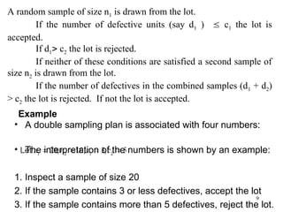
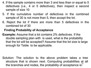
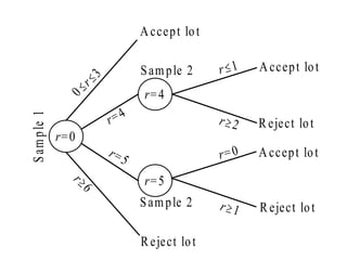
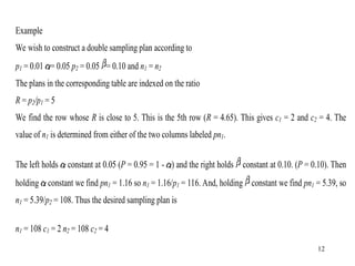
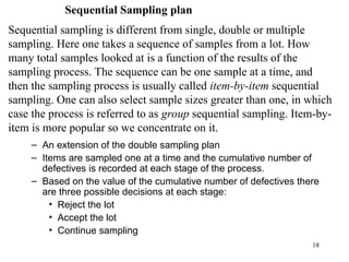
1. 1
Chapter Three
Acceptance Sampling
Outline
• Sampling
• Some sampling plans
• A single sampling plan
• Double and Multiple sample plan
• Sequential sample plan
• Some definitions

2. 2
Acceptance sampling is a method used to accept or reject
product based on a random sample of the product.
The purpose of acceptance sampling is to judgment lots (accept
or reject) rather than to estimate the quality of a lot.
Acceptance sampling plans do not improve quality. The nature
of sampling is such that acceptance sampling will accept some
lots and reject others even though they are of the same quality.
The most effective use of acceptance sampling is as an auditing tool
to help ensure that the output of a process meets requirements.
As mentioned acceptance sampling can reject “good” lots and accept
“bad” lots. More formally:

3. 3
Necessity of Sampling
• In most cases 100% inspection is too costly.
• In some cases 100% inspection may be impossible.
• If only the defective items are returned, repair or
replacement may be cheaper than improving quality.
But, if the entire lot is returned on the basis of sample
quality, then the producer has a much greater
motivation to improve quality.

4. 4
Some Sampling Plans
• Single sampling plans:
– Most popular and easiest to use
– Two numbers n and c
– If there are more than c defectives in a sample of size n
the lot is rejected; otherwise it is accepted
• Double sampling plans:
– A sample of size n1 is selected.
– If the number of defectives is less than or equal to c1
than the lot is accepted.
– Else, another sample of size n2 is drawn.
– If the cumulative number of defectives in both samples
is more than c2 the lot is rejected; otherwise it is
accepted.

5. 5

6. 6

7. 7
If lots inspected are 2% defective, the probability of accepting the
lot, with this sampling plan, is .7366. This means that if 100 lots
are manufacture with 2% defective we will accept 74 lots and
reject 26.

8. 8
• Double Sampling Plan
• A double sampling plan is more difficult to
construct and more difficult to implement
than a single sampling plan. However, it
has the following advantages:
–A double sampling plan may give similar
levels of the consumer’s and the
producer’s risk but require less sampling
in the long run than a single sampling
plan

9. 9
Example
• A double sampling plan is associated with four numbers:
• The interpretation of the numbers is shown by an example:
1. Inspect a sample of size 20
2. If the sample contains 3 or less defectives, accept the lot
3. If the sample contains more than 5 defectives, reject the lot.
A random sample of size n1 is drawn from the lot.
If the number of defective units (say d1 )  c1 the lot is
accepted.
If d1 c2 the lot is rejected.
If neither of these conditions are satisfied a second sample of
size n2 is drawn from the lot.
If the number of defectives in the combined samples (d1 + d2)
> c2 the lot is rejected. If not the lot is accepted.

10. 10
4. If the sample contains more than 3 and less than or equal to 5
defectives (i.e., 4 or 5 defectives), then inspect a second
sample of size 10
5. If the cumulative number of defectives in the combined
sample of 30 is not more than 5, then accept the lot.
6. Reject the lot if there are more than 5 defectives in the
combined lot of 30
Finding Probability of Acceptance
Example: Assume that a lot contains 2% defectives. If the
double sampling plan with is used, what is the probability
that the lot will be accepted? Assume that the lot size is large
enough for Table to be applicable.
Solution: The solution to the above problem takes a tree
structure that is shown next. Computing probabilities at all
the branches and nodes, the probability of acceptance is:

11. 11
r=0
S
a
m
p
le
1
r=4
r=5
Sample 2
Sample 2
Accept lot
Reject lot
Accept lot
Accept lot
Reject lot
Reject lot

12. 12
Example
We wish to construct a double sampling plan according to
p1 = 0.01 = 0.05 p2 = 0.05 = 0.10 and n1 = n2
The plans in the corresponding table are indexed on the ratio
R = p2/p1 = 5
We find the row whose R is close to 5. This is the 5th row (R = 4.65). This gives c1 = 2 and c2 = 4. The
value of n1 is determined from either of the two columns labeled pn1.
The left holds constant at 0.05 (P = 0.95 = 1 - ) and the right holds constant at 0.10. (P = 0.10). Then
holding constant we find pn1 = 1.16 so n1 = 1.16/p1 = 116. And, holding constant we find pn1 = 5.39, so
n1 = 5.39/p2 = 108. Thus the desired sampling plan is
n1 = 108 c1 = 2 n2 = 108 c2 = 4

13. 13
Tables for n1 = n2
accept approximation values
R = numbers of pn1 for
p2/p1 c1 c2 P = .95 P = .10
11.90 0 1 0.21 2.50
7.54 1 2 0.52 3.92
6.79 0 2 0.43 2.96
5.39 1 3 0.76 4.11
4.65 2 4 1.16 5.39
4.25 1 4 1.04 4.42
3.88 2 5 1.43 5.55
3.63 3 6 1.87 6.78
3.38 2 6 1.72 5.82
3.21 3 7 2.15 6.91
3.09 4 8 2.62 8.10
2.85 4 9 2.90 8.26
2.60 5 11 3.68 9.56
2.44 5 12 4.00 9.77
2.32 5 13 4.35 10.08
2.22 5 14 4.70 10.45
2.12 5 16 5.39 11.41

14. 14
Multiple Sampling Plan
Finding Probability of Acceptance
• Double sampling plans may be extended to triple sampling
plans, which may also be extended to higher order plans.
The logical conclusion of this process is the multiple or
sequential sampling plan.
• Multiple sampling and sequential sampling are very
similar. Usually, in a multiple sampling plan the decisions
(regarding accept/reject/continue) are made after each lot
is sampled. On the other hand, in a sequential sampling
plan, the decisions are made after each item is sampled.
In a multiple sampling 3 or more samples are taken. A
sequential sampling may not have any limit on the number
of items inspected.

15. 15
Multiple sampling plans
Multiple sampling: - is an extension of double sampling. It involves inspection of 1 to k successive samples
as required. Multiple sampling plans are usually presented in tabular form: The procedure commences with
taking a random sample of size n1 from a large lot of size N and counting the number of defectives, d1.
If d1 a1 the lot is accepted.
If d1 r1 the lot is rejected.
If a1 < d1 < r1, another sample is taken.
Stage Sample Size Acceptance Number Rejection Number
1 n1 Ac1 Re1
2 n2 Ac2 Re2
3 n3 Ac3 Re3
. . . .
. . . .
. . . .
M nm Acm Rem( = Acm+1)

16. 16
Problem 3 : A multiple sampling plan is as follows:
Sample Individual Combined Acceptance Rejection
Number Sample Size Sample Size Number Number
1 5 5 -- 2
2 5 10 0 2
3 5 15 1 3
4 5 20 2 3
Assuming that lot size is large enough for Table to be
applicable, compute the probability of acceptance of a 10%
defective lot.
ASN= n1p1+ (n1+n2) (1-p1)
=n1+n2 (1-p1)

17. 17
r=0 r=1
r2
r=0
r=1
r2
r=0
Reject Reject
Accept
r=2
r3
r=1
Reject
r=2
r3
Reject
Accept
Accept

18. 18
Sequential sampling is different from single, double or multiple
sampling. Here one takes a sequence of samples from a lot. How
many total samples looked at is a function of the results of the
sampling process. The sequence can be one sample at a time, and
then the sampling process is usually called item-by-item sequential
sampling. One can also select sample sizes greater than one, in which
case the process is referred to as group sequential sampling. Item-by-
item is more popular so we concentrate on it.
Sequential Sampling plan
– An extension of the double sampling plan
– Items are sampled one at a time and the cumulative number of
defectives is recorded at each stage of the process.
– Based on the value of the cumulative number of defectives there
are three possible decisions at each stage:
• Reject the lot
• Accept the lot
• Continue sampling

19. 19

20. 20
The cumulative observed number of defectives is plotted on the
graph. For each point, the x-axis is the total number of items thus far
selected, and the y-axis is the total number of observed defectives. If
the plotted point falls within the parallel lines the process continues
by drawing another sample. As soon as a point falls on or above the
upper line, the lot is rejected. And when a point falls on or below the
lower line, the lot is accepted. The process can theoretically last
until the lot is 100% inspected. However, as a rule of thumb,
sequential-sampling plans are truncated after the number inspected
reaches three times the number that would have been inspected
using a corresponding single sampling plan

21. 21
As an example, let p1 = .01, p2 = .10, = .05, = .10. The resulting equations are
Both acceptance numbers and rejection numbers must be integers. The acceptance number is the next
integer less than or equal to xa and the rejection number is the next integer greater than or equal to xr. Thus
for n = 1, the acceptance number = -1, which is impossible, and the rejection number = 2, which is also
impossible. For n = 24, the acceptance number is 0 and the rejection number = 3.
The results for n =1, 2, 3... 26 are tabulated below.

22. 22
n
inspect
n
accept
n
reject
n
inspect
n
accept
n
reject
1 x x 14 x 2
2 x 2 15 x 2
3 x 2 16 x 3
4 x 2 17 x 3
5 x 2 18 x 3
6 x 2 19 x 3
7 x 2 20 x 3
8 x 2 21 x 3
9 x 2 22 x 3
10 x 2 23 x 3
11 x 2 24 0 3
12 x 2 25 0 3
13 x 2 26 0 3
So, for n = 24 the acceptance number is 0 and the rejection
number is 3. The "x" means that acceptance or rejection is
not possible.