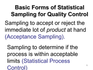
The document discusses two main types of statistical sampling for quality control: acceptance sampling and statistical process control. Acceptance sampling involves inspecting finished products to determine whether to accept or reject the entire lot, while statistical process control involves sampling processes to determine if they are operating within acceptable limits. The document then provides more details on acceptance sampling, including its purposes and advantages, how acceptance sampling plans are designed, typical applications of acceptance sampling, and how operating characteristic curves are used to calculate acceptance sampling plans.

1. Basic Forms of Statistical
Sampling for Quality Control
Sampling to accept or reject the
immediate lot of product at hand
(Acceptance Sampling).
Sampling to determine if the
process is within acceptable
limits (Statistical Process
1
Control)

2. ACCEPTANCE SAMPLING (AS)
• INSPECTION AFTER PRODUCTION.
• HOWEVER - SHOULD NOT TRY TO
INSPECT QUALITY INTO PRODUCT.
• AS IS AN AUDITING TOOL.
2

3. Acceptance Sampling
• Purposes
– Determine quality level
– Ensure quality is within predetermined level
• Advantages
– Economy
– Less handling damage
– Fewer inspectors
– Upgrading of the inspection job
– Applicability to destructive testing
– Entire lot rejection (motivation for improvement)
3

4. DESIGNING THE PLAN
• Acceptable Quality Level (AQL) = Max.
acceptable percentage of defectives defined
by producer.
• α (Producer’s risk) = The probability of
rejecting a good lot.
• Limiting Quality Level (LQL) = Lot
Tolerance Percent Defective (LTPD) =
Percentage of defectives that defines
consumer’s rejection point.
• Β (Consumer’s risk) =The probability of
accepting a bad lot. 4

5. Typical Application of
Acceptance Sampling
• The decision to accept or reject the
shipment is based on the following set
standards:
– Lot size = N
– Sample size = n
– Acceptance number = c
– Defective items = d
• If d <= c, accept lot
• If d > c, reject lot

6. OC Curve Calculation
• Two Ways of Calculating OC Curves
– Binomial Distribution
– Poisson formula
• Binomial Distribution
– Cannot use because:
• Binomials are based on constant probabilities.
• N is not infinite
• p changes

7. OC Curve Calculation
• A Poisson formula can be used
• Poisson is a limit
– Limitations of using Poisson
• n<= 1/10 total batch N
• Little faith in probability calculation when n is quite
small and p quite large.
.

8. Calculation of OC Curve
• Find your sample size, n
• Find your fraction defect p
• Multiply n*p
• A=d
• From a Poisson table find your PA

9. Calculation of an OC Curve
• N = 1000 Np d= 3
• n = 60 .6 99.8
• p = .01 1.2 87.9
• A=3 3 64.7
• Find PA for p = .01, .
4.2 39.5
02, .05, .07, .1, and .
12? 6 151
7.2 072

10. Properties of OC Curves
• Ideal curve would be
perfectly
perpendicular from 0
to 100% for a given
fraction defective.

11. Properties of OC Curves
• The acceptance number and sample
size are most important factors.
• Decreasing the acceptance number is
preferred over increasing sample size.
• The larger the sample size the steeper
the curve.

12. Properties of OC Curves

13. Properties of OC Curves
• By changing the
acceptance level, the
shape of the curve
will change. All
curves permit the
same fraction of
sample to be
nonconforming.

14. Operating Characteristics (OC)
Curves
• OC curves are graphs which
show the probability of accepting
a lot given various proportions of
defects in the lot
• X-axis shows % of items that are
defective in a lot- “lot quality”
• Y-axis shows the probability or
chance of accepting a lot
• As proportion of defects
increases, the chance of
accepting lot decreases
• Example: 90% chance of
accepting a lot with 5%
defectives; 10% chance of
accepting a lot with 24%
defectives

15. AQL, LTPD, Consumer’s Risk (α) &
Producer’s Risk (β)
• AQL is the small % of defects that
consumers are willing to accept;
order of 1-2%
• LTPD is the upper limit of the
percentage of defective items
consumers are willing to tolerate
• Consumer’s Risk (α) is the chance
of accepting a lot that contains a
greater number of defects than the
LTPD limit; Type II error
• Producer’s risk (β) is the chance a
lot containing an acceptable quality
level will be rejected; Type I error

16. Developing OC Curves
• OC curves graphically depict the discriminating power
of a sampling plan
• Cumulative binomial tables like partial table below are
used to obtain probabilities of accepting a lot given
varying levels of lot defectives
• Top of the table shows value of p (proportion of
defective items in lot), Left hand column shows values
of n (sample size) and x represents the cumulative
number of defects found

17. Constructing an OC Curve
• Lets develop an OC curve for a
sampling plan in which a sample
of 5 items is drawn from lots of
N=1000 items
• The accept /reject criteria are set
up in such a way that we accept
a lot if no more that one defect
(c=1) is found
• Note that we have a 99.74%
chance of accepting a lot with
5% defects and a 73.73% chance
with 20% defects

18. Average Outgoing Quality (AOQ)
• With OC curves, the higher the quality
of the lot, the higher is the chance that
it will be accepted
• Conversely, the lower the quality of the
lot, the greater is the chance that it will
be rejected
• The average outgoing quality level of
the product (AOQ) can be computed as
follows: AOQ=(Pac)p
• AOQ can be calculated for each
proportion of defects in a lot by using
the above equation
• This graph is for n=5 and x=1 (same
as c=1)
• AOQ is highest for lots close to 30%
defects

19. Implications for Managers
• How much and how often to inspect?
– Consider product cost and product volume
– Consider process stability
– Consider lot size
• Where to inspect?
– Inbound materials
– Finished products
– Prior to costly processing
• Which tools to use?
– Control charts are best used for in-process production
– Acceptance sampling is best used for
inbound/outbound

20. OC Curves
100%
OC Curves come in
various shapes
depending on the
Probability of Accepting Lot
75%
sample size and risk of
α and β errors
50% This curve is more
discriminating
25% This curve is less
discriminating
.03 .06 .09
Lot Quality (Fraction Defective)

21. OC Definitions on the Curve
100%
α = 0.10
90%
Probability of Accepting Lot
75%
50%
25%
LTPD
AQL
Go
β = 0.10 od Indifferent Bad
.03 .06 .09
Lot Quality (Fraction Defective)

22. DEFINING GOOD AND BAD
SHIPMENTS: AQL VERSUS LTPD
• Instead of simply "good" versus "bad", we will
define "really good", "really bad", and "ok, but not
great" shipments
– A really good shipment has p <= AQL
– A really bad shipment has p >= LTPD
– Anything in between (AQL < p < LTPD) is ok, but not
great

23. THE OPERATING-
CHARACTERISTIC (OC) CURVE
• For a given a sampling plan and a specified true
fraction defective p, we can calculate
– Pa -- Probability of accepting lot
• If lot is truly good, 1 - Pa = α
• If lot is truly bad, Pa = β
• A plot of Pa as a function of p is called the OC
curve for a given sampling plan

24. THE OPERATING-
CHARACTERISTIC (OC) CURVE
• The ideal sampling plan discriminates perfectly
between good and bad shipments
– Both α and β are zero in this example!
– This requires a sample size equal to the population -- not
feasible
1.0
Pa
0.0
GOOD BAD
p

25. USING AN OC CURVE
• How do we find α and β using an OC curve?
– AQL = 0.01
– LTPD = 0.05
• Then α = 1 – Pa(p=0.01) = 1 - 0.9206 = 0.0794
• And β = Pa(p=0.05) = 0.1183

26. AVERAGE OUTGOING QUALITY
• Consider a part with a long-term fraction
nonconforming of p
– Samples of size n are taken from a lot of size N and
inspected
– Any defectives in the sample of size n are replaced,
accept or reject
• When a lot of is accepted, we expect p(N-n)
defectives in the remainder of the lot
• When a lot is rejected, it will be sorted and
defective units replaced, leaving N-n good units in
the remainder
• This is referred to as "rectifying" inspection

27. AVERAGE OUTGOING QUALITY
• If Pa is the probability of accepting a lot, then the
average outgoing quality is:
Pap( N − n )
AOQ =
N
0.9859(0.005)(10000 − 100)
AOQ = = 0.0049
10000
• The worst possible AOQ is the AOQ Limit or AOQL

28. AVERAGE TOTAL INSPECTION
• Rectifying plans have greater inspection
requirements
• The Average Total Inspections:
ATI = n + (1 − Pa )( N − n )
ATI = 100 + (1 − 0.9859)(10000 − 100) = 240

29. Types of Acceptance sampling
Plans
Single-sampling plan
Double-sampling plan
Multiple-sampling plan
Sequential-sampling plan

30. Single-sampling plan
Total number ： N
The proportion of defects :P
Acc the lot
S n <C
(N, p) (n,c)
S n >C Reject the lot
Where Sn is the number of the actual defects in the sample.

31. DOUBLE SAMPLING PLANS
• Define:
– n1 -- sample size on first sample
– c1 -- acceptance number for first sample
– d1 -- defectives in first sample
– n2 -- sample size on second sample
– c2 -- acceptance number for both samples
– d2 -- defectives in second sample
• Take sample of size n1
– Accept if d1 ≤ c1; reject if d1 > c2;
– Take second sample of size n2 if c1 < d1 ≤ c2
– Accept if d1+d2 ≤ c2; reject if d1+d2 > c2

32. Multiple-sampling plan
Acc the lot S Acc the lot
S n1 <c 1 (n1+n2) <r 2
c 2 <S (n1+n2) <r 2
c 1 <Sn 1 <r 1 (n 1 +n 2 +n 3 ) ……..
(n,p) (n 1 +n 2 )
S (n1+n2) >r 2
S n1 >c 1
Reject the lot Reject the lot

34. Sequential Sampling Plan

35.  producer ' s risk ≤ α OC ( P ) ≥ 1 − α
1
 ⇒
Consumer ' s risk ≤ β  OC ( P2 ) ≤ β
Example:
AQL=1 %
α = 0.05;
LQL=6 %
OC (1%)=0.95 β = 0.10
OC(6 %)=0.10
(n,c)=(89, 2)

36. n ,c’s effect on OC-Curve

37. Example: Acceptance Sampling
Problem
Zypercom, a manufacturer of video interfaces,
purchases printed wiring boards from an outside
vender, Procard. Procard has set an acceptable
quality level of 1% and accepts a 5% risk of rejecting
lots at or below this level. Zypercom considers lots
with 3% defectives to be unacceptable and will
assume a 10% risk of accepting a defective lot.
Develop a sampling plan for Zypercom and
determine a rule to be followed by the receiving
inspection personnel.

38. Example: Step 1. What is given
and what is not?
In this problem, AQL is given to be 0.01 and LTDP is given to be
0.03. We are also given an alpha of 0.05 and a beta of 0.10.
What you need to determine
your sampling plan is “c” and
“n.”

39. Example: Step 2. Determine “c”
LTPD .03
First divide LTPD by AQL. = = 3
AQL .01
Then find the value for “c” by selecting the value in the Table
“n(AQL)”column that is equal to or just greater than the ratio above.
Exhibit
Exhibit So, c = 6.
c LTPD/AQL n AQL c LTPD/AQL n AQL
0 44.890 0.052 5 3.549 2.613
1 10.946 0.355 6 3.206 3.286
2 6.509 0.818 7 2.957 3.981
3 4.890 1.366 8 2.768 4.695
4 4.057 1.970 9 2.618 5.426

40. Example: Step 3. Determine
Sample Size
Now given the information below, compute the sample size
in units to generate your sampling plan.
c = 6, from Table
n (AQL) = 3.286, from Table
AQL = .01, given in problem
n(AQL/AQL) = 3.286/.01 = 328.6, or 329 (always round up)
Sampling Plan:
Take a random sample of 329 units from a lot.
Reject the lot if more than 6 units are defective.

41. TYPES OF INSP. AND
SWITCHING
• STD. PLANS FACILITATE
CONDITIONAL INSPECTIONS
• NORMAL - WITH NORMAL LEVEL OF
DEFECTS
• TIGHTENED - WITH HIGH LEVEL OF
DEFECTS
• REDUCED - WITH OUTPUT
REDUCED DEFECTS

42. SWITCHING RULES
• N > T (NORMAL TO TIGHTENED)
• T>N
• N>R
• R>N
• DISCONTINUANCE BECAUSE OF
POOR QUALITY

43. ISO 2859 (ANSI/ASQC Z1.4)
• One of oldest sampling systems
– Covers single, double, & multiple sampling
– AQL-based: Type I error ranges 9%-1% as sample size
increases
– Minimal control over Type II error
– Type II error decreases as general inspection level (I, II,
III) increases
– “Special” inspection levels when small samples needed
(and high Type II error probability tolerated)
• Mechanism for reduced or tightened inspection
depending on recent vendor performance
– Tightened -- more inspection
– Reduced -- less inspection

44. ISO 2859 (ANSI/ASQC Z1.4)
• A vendor begins at a "normal" inspection level
– Normal to tightened: 2/5 lots rejected
– Normal to reduced:
• Previous 10 lots accepted (NOT ISO 2859)
• Total defectives from 10 lots ok (NOT ISO 2859)
• If a vendor is at a tightened level:
– Tightened to normal: 5 previous lots accepted
• If a vendor is at a reduced level:
– Reduced to normal: a lot is rejected

45. ISO 2859
• A vendor begins at a "normal" inspection
level
– Normal to reduced:
• “Switching score” set to zero
• If acceptance number is 0 or 1:
– Add 3 to the score if the lot would still have been
accepted with an AQL one step tighter; else reset score
to 0
• If acceptance number is 2 or more:
– Add 3 to the score if the lot is accepted; else reset
score to 0
• If score hits 30, switch to reduced inspection

46. USING ISO 2859
1. Choose the AQL
2. Choose the general inspection level
3. Determine lot size
4. Find sample size code
5. Choose type of sampling plan
6. Select appropriate plan from table
7. Switch to reduced/tightened inspection as
required

47. USING ISO 2859

48. USING ISO 2859

49. USING ISO 2859

50. USING ISO 2859

51. DODGE-ROMIG PLANS
• Developed in the 1920's
• Rectifying plans
• Requires knowledge of vendor's long-term
process average (fraction non-conforming)
• Choice of LTPD or AOQL orientation
– Both minimize ATI for specified process average
– Type II error = 10%,

52. DODGE-ROMIG PLANS
• AOQL plans:
– 1) Determine N, p, and AOQL
– 2) Use table to find n and c
– Finds plan with specified AOQL which minimizes ATI
– Calculate resulting LTPD with Type II error = 10%
• LTPD plans:
– 1) Determine N, p, and LTPD
– 2) Use table to find n and c
– Finds plan with specified LTPD which minimizes ATI
– Calculate resulting AOQL

53. DODGE-ROMIG PLANS

54. DODGE-ROMIG PLANS