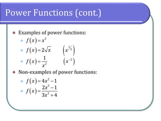
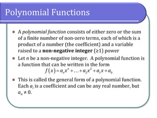
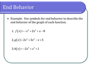
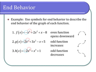
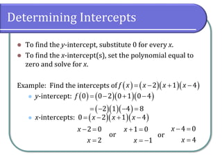
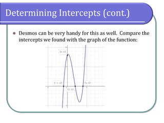
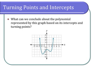
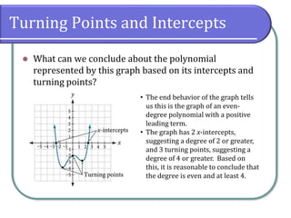
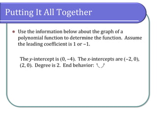
5.2 Power Functions &
Polynomial Functions
Chapter 5 Polynomial and Rational Functions
Concepts and Objectives
⚫ Objectives for the section are
⚫ Identify power functions.
⚫ Identify end behavior of power functions.
⚫ Identify polynomial functions.
⚫ Identify the degree and leading coefficient of
polynomial functions.
Power Functions
⚫ A power function is a function with a single term that is
the product of a real number (the coefficient) and a
variable raised to a fixed real number.
⚫ It can be represented in the form
where k and p are real numbers.
( )= ,
p
f x kx
Power Functions (cont.)
⚫ Examples of power functions:
⚫
⚫
⚫
⚫ Non-examples of power functions:
⚫
⚫
( ) 3
f x x
=
( ) 2
f x x
= ( )
1
2
x
( ) 2
1
f x
x
= ( )
2
x−
( ) 2
4 1
f x x
= −
( )
5
2
2 1
3 4
x
f x
x
−
=
+
Polynomial Functions
⚫ A polynomial function consists of either zero or the sum
of a finite number of non-zero terms, each of which is a
product of a number (the coefficient) and a variable
raised to a non-negative integer (≥1) power
⚫ Let n be a non-negative integer. A polynomial function is
a function that can be written in the form
⚫ This is called the general form of a polynomial function.
Each ai is a coefficient and can be any real number, but
an ≠ 0.
( ) 2
2 1 0
n
n
f x a x a x a x a
= + + + +
Polynomial Functions (cont.)
⚫ Polynomial functions are different from power functions
in that
⚫ they can consist of multiple terms combined by
addition or subtraction
⚫ their exponents must be non-negative integers
The Degree and Leading Term
⚫ The degree of a polynomial (or power) function is the
highest power of the variable that occurs in the
polynomial.
⚫ The leading term is the term containing the highest
power of the variable.
⚫ The leading coefficient is the coefficient of the leading
term.
⚫ The leading term does not have to be the first term in
the polynomial.
Identifying the Degree and Leading
Coefficient
Examples: Identify the degree and the leading coefficient
of the following polynomial functions.
⚫ f
⚫
⚫
( ) 5 3
6 2 7
f t t t t
= − +
( ) 2 3
3 2 4
g x x x
= + −
( ) 3
6 2
h p p p
= − −
Identifying the Degree and Leading
Coefficient
Examples: Identify the degree and the leading coefficient
of the following polynomial functions.
⚫ f
Degree: 5 Leading coefficient: 6
⚫
Degree: 3 Leading coefficient: ‒4
⚫
Degree: 3 Leading coefficient: ‒1
( ) 5 3
6 2 7
f t t t t
= − +
( ) 2 3
3 2 4
g x x x
= + −
( ) 3
6 2
h p p p
= − −
Graphs of Polynomial Functions
⚫ If we look at graphs of functions of the form ,
we can see a definite pattern:
( )= n
f x ax
( )= 2
f x x ( )= 3
g x x
( )= 4
h x x ( )= 5
j x x
End Behavior
⚫ The end behavior of a polynomial graph is determined by
the leading term (also called the dominating term).
⚫ For example, has the same end
behavior as once you zoom out far enough.
( )= − +
3
2 8 9
f x x x
( )= 3
2
f x x
End Behavior
⚫ Example: Use symbols for end behavior to describe the
end behavior of the graph of each function.
1.
2.
3.
( )= − + + −
4 2
2 8
f x x x x
( )= + − +
3 2
2 3 5
g x x x x
( )= − + +
5 3
2 1
h x x x
End Behavior
⚫ Example: Use symbols for end behavior to describe the
end behavior of the graph of each function.
1.
2.
3.
( )= − + + −
4 2
2 8
f x x x x even function
opens downward
( )= + − +
3 2
2 3 5
g x x x x odd function
increases
( )= − + +
5 3
2 1
h x x x odd function
decreases
Turning Points and Intercepts
⚫ The point where a graph changes direction (“bounces”
or “wiggles”) is called a turning point of the function.
⚫ The y-intercept is the point at which the function has an
input value of zero.
⚫ The x-intercepts are the points at which the output value
is zero.
Determining Intercepts
⚫ To find the y-intercept, substitute 0 for every x.
⚫ To find the x-intercept(s), set the polynomial equal to
zero and solve for x.
Example: Find the intercepts of
⚫ y-intercept:
⚫ x-intercepts:
( ) ( )( )( )
2 1 4
f x x x x
= − + −
( ) ( )( )( )
( )( )( )
0 0 2 0 1 0 4
2 1 4 8
f = − + −
= − − =
( )( )( )
0 2 1 4
x x x
= − + −
2 0
2
x
x
− =
=
or
1 0
1
x
x
+ =
= −
or
4 0
4
x
x
− =
=
Determining Intercepts (cont.)
⚫ Desmos can be very handy for this as well. Compare the
intercepts we found with the graph of the function:
Turning Points and Intercepts
⚫ A polynomial function of degree n will have at most
n x-intercepts and n – 1 turning points, with at least one
turning point between each pair of adjacent zeros.
(Because it is a function, there is only one y-intercept.)
⚫ Example: Without graphing the function, determine the
local behavior of the function by finding the maximum
number of x-intercepts and turning points for
⚫ The polynomial has a degree of 10, so there are at
most 10 x-intercepts and at most 9 turning points.
( ) 10 7 4 3
3 4 2
f x x x x x
= − + − +
Turning Points and Intercepts
⚫ What can we conclude about the polynomial
represented by this graph based on its intercepts and
turning points?
Turning Points and Intercepts
⚫ What can we conclude about the polynomial
represented by this graph based on its intercepts and
turning points?
• The end behavior of the graph tells
us this is the graph of an even-
degree polynomial with a positive
leading term.
• The graph has 2 x-intercepts,
suggesting a degree of 2 or greater,
and 3 turning points, suggesting a
degree of 4 or greater. Based on
this, it is reasonable to conclude that
the degree is even and at least 4.
Putting It All Together
⚫ Use the information below about the graph of a
polynomial function to determine the function. Assume
the leading coefficient is 1 or ‒1.
The y-intercept is (0, ‒4). The x-intercepts are (‒2, 0),
(2, 0). Degree is 2. End behavior:
Putting It All Together
⚫ Use the information below about the graph of a
polynomial function to determine the function. Assume
the leading coefficient is 1 or ‒1.
The y-intercept is (0, ‒4). The x-intercepts are (‒2, 0),
(2, 0). Degree is 2. End behavior:
( ) ( )( )
2 2
f x x x
= + −
Classwork
⚫ College Algebra 2e
⚫ 5.2: 12-24 (even); 5.1: 26-32, 40-44 (even); 4.3: 32-
42 (even)
⚫ 5.2 Classwork Check
⚫ Quiz 5.1

5.2 Power Functions and Polynomial Functions

  • 1.
    5.2 Power Functions& Polynomial Functions Chapter 5 Polynomial and Rational Functions
  • 2.
    Concepts and Objectives ⚫Objectives for the section are ⚫ Identify power functions. ⚫ Identify end behavior of power functions. ⚫ Identify polynomial functions. ⚫ Identify the degree and leading coefficient of polynomial functions.
  • 3.
    Power Functions ⚫ Apower function is a function with a single term that is the product of a real number (the coefficient) and a variable raised to a fixed real number. ⚫ It can be represented in the form where k and p are real numbers. ( )= , p f x kx
  • 4.
    Power Functions (cont.) ⚫Examples of power functions: ⚫ ⚫ ⚫ ⚫ Non-examples of power functions: ⚫ ⚫ ( ) 3 f x x = ( ) 2 f x x = ( ) 1 2 x ( ) 2 1 f x x = ( ) 2 x− ( ) 2 4 1 f x x = − ( ) 5 2 2 1 3 4 x f x x − = +
  • 5.
    Polynomial Functions ⚫ Apolynomial function consists of either zero or the sum of a finite number of non-zero terms, each of which is a product of a number (the coefficient) and a variable raised to a non-negative integer (≥1) power ⚫ Let n be a non-negative integer. A polynomial function is a function that can be written in the form ⚫ This is called the general form of a polynomial function. Each ai is a coefficient and can be any real number, but an ≠ 0. ( ) 2 2 1 0 n n f x a x a x a x a = + + + +
  • 6.
    Polynomial Functions (cont.) ⚫Polynomial functions are different from power functions in that ⚫ they can consist of multiple terms combined by addition or subtraction ⚫ their exponents must be non-negative integers
  • 7.
    The Degree andLeading Term ⚫ The degree of a polynomial (or power) function is the highest power of the variable that occurs in the polynomial. ⚫ The leading term is the term containing the highest power of the variable. ⚫ The leading coefficient is the coefficient of the leading term. ⚫ The leading term does not have to be the first term in the polynomial.
  • 8.
    Identifying the Degreeand Leading Coefficient Examples: Identify the degree and the leading coefficient of the following polynomial functions. ⚫ f ⚫ ⚫ ( ) 5 3 6 2 7 f t t t t = − + ( ) 2 3 3 2 4 g x x x = + − ( ) 3 6 2 h p p p = − −
  • 9.
    Identifying the Degreeand Leading Coefficient Examples: Identify the degree and the leading coefficient of the following polynomial functions. ⚫ f Degree: 5 Leading coefficient: 6 ⚫ Degree: 3 Leading coefficient: ‒4 ⚫ Degree: 3 Leading coefficient: ‒1 ( ) 5 3 6 2 7 f t t t t = − + ( ) 2 3 3 2 4 g x x x = + − ( ) 3 6 2 h p p p = − −
  • 10.
    Graphs of PolynomialFunctions ⚫ If we look at graphs of functions of the form , we can see a definite pattern: ( )= n f x ax ( )= 2 f x x ( )= 3 g x x ( )= 4 h x x ( )= 5 j x x
  • 11.
    End Behavior ⚫ Theend behavior of a polynomial graph is determined by the leading term (also called the dominating term). ⚫ For example, has the same end behavior as once you zoom out far enough. ( )= − + 3 2 8 9 f x x x ( )= 3 2 f x x
  • 12.
    End Behavior ⚫ Example:Use symbols for end behavior to describe the end behavior of the graph of each function. 1. 2. 3. ( )= − + + − 4 2 2 8 f x x x x ( )= + − + 3 2 2 3 5 g x x x x ( )= − + + 5 3 2 1 h x x x
  • 13.
    End Behavior ⚫ Example:Use symbols for end behavior to describe the end behavior of the graph of each function. 1. 2. 3. ( )= − + + − 4 2 2 8 f x x x x even function opens downward ( )= + − + 3 2 2 3 5 g x x x x odd function increases ( )= − + + 5 3 2 1 h x x x odd function decreases
  • 14.
    Turning Points andIntercepts ⚫ The point where a graph changes direction (“bounces” or “wiggles”) is called a turning point of the function. ⚫ The y-intercept is the point at which the function has an input value of zero. ⚫ The x-intercepts are the points at which the output value is zero.
  • 15.
    Determining Intercepts ⚫ Tofind the y-intercept, substitute 0 for every x. ⚫ To find the x-intercept(s), set the polynomial equal to zero and solve for x. Example: Find the intercepts of ⚫ y-intercept: ⚫ x-intercepts: ( ) ( )( )( ) 2 1 4 f x x x x = − + − ( ) ( )( )( ) ( )( )( ) 0 0 2 0 1 0 4 2 1 4 8 f = − + − = − − = ( )( )( ) 0 2 1 4 x x x = − + − 2 0 2 x x − = = or 1 0 1 x x + = = − or 4 0 4 x x − = =
  • 16.
    Determining Intercepts (cont.) ⚫Desmos can be very handy for this as well. Compare the intercepts we found with the graph of the function:
  • 17.
    Turning Points andIntercepts ⚫ A polynomial function of degree n will have at most n x-intercepts and n – 1 turning points, with at least one turning point between each pair of adjacent zeros. (Because it is a function, there is only one y-intercept.) ⚫ Example: Without graphing the function, determine the local behavior of the function by finding the maximum number of x-intercepts and turning points for ⚫ The polynomial has a degree of 10, so there are at most 10 x-intercepts and at most 9 turning points. ( ) 10 7 4 3 3 4 2 f x x x x x = − + − +
  • 18.
    Turning Points andIntercepts ⚫ What can we conclude about the polynomial represented by this graph based on its intercepts and turning points?
  • 19.
    Turning Points andIntercepts ⚫ What can we conclude about the polynomial represented by this graph based on its intercepts and turning points? • The end behavior of the graph tells us this is the graph of an even- degree polynomial with a positive leading term. • The graph has 2 x-intercepts, suggesting a degree of 2 or greater, and 3 turning points, suggesting a degree of 4 or greater. Based on this, it is reasonable to conclude that the degree is even and at least 4.
  • 20.
    Putting It AllTogether ⚫ Use the information below about the graph of a polynomial function to determine the function. Assume the leading coefficient is 1 or ‒1. The y-intercept is (0, ‒4). The x-intercepts are (‒2, 0), (2, 0). Degree is 2. End behavior:
  • 21.
    Putting It AllTogether ⚫ Use the information below about the graph of a polynomial function to determine the function. Assume the leading coefficient is 1 or ‒1. The y-intercept is (0, ‒4). The x-intercepts are (‒2, 0), (2, 0). Degree is 2. End behavior: ( ) ( )( ) 2 2 f x x x = + −
  • 22.
    Classwork ⚫ College Algebra2e ⚫ 5.2: 12-24 (even); 5.1: 26-32, 40-44 (even); 4.3: 32- 42 (even) ⚫ 5.2 Classwork Check ⚫ Quiz 5.1