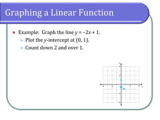
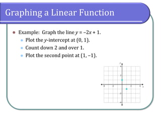
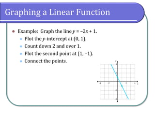
Linear Functions
Chapter 2 Graphs and Functions
Concepts & Objectives
⚫ Function Properties
⚫ Identify whether a relation is a function
⚫ Identify the domain and range of a given function
⚫ Linear Functions
⚫ Calculate the slope between two points
⚫ Graph a linear function
Functions
⚫ A relation is a set of ordered pairs.
⚫ A function is a relation in, for each distinct value of the
first component of the ordered pairs, there is exactly one
value of the second component.
⚫ More formally:
If A and B are sets, then a function f from A to B
(written f: A → B)
is a rule that assigns to each element of A
a unique element of set B.
Functions (cont.)
⚫ The set A is called the domain of the function f
⚫ Every element of A must be included in the function.
⚫ The set B is called the codomain of f
⚫ The subset of B consisting of those elements that are
images under the function f is called the range.
⚫ The range and the codomain may or may not be the
same.
Functions (cont.)
⚫ In terms of ordered pairs, a function is the set of ordered
pairs (A, f (A)).
⚫ Historical note: The notation f (x) for a function of a
variable quantity x was introduced in 1748 by Leonhard
Euler in his text Algebra, which was the forerunner of
today’s algebra texts. Many other mathematical symbols
in use today (such as e and ) were introduced by Euler
in his writings.
Functions (cont.)
⚫ For the most part, we use f (x) and y interchangeably to
denote a function of x, but there are some subtle
differences.
⚫ y is the output variable, while f (x) is the rule that
produces the output variable.
⚫ An equation with two variables, x and y, may not be a
function at all.
Example: is a circle, but not a function+ =2 2
4x y
Linear Functions
⚫ A function f is a linear function if, for a and b  ,
⚫ If a ≠ 0, the domain and the range of a linear function are
both .
⚫ The slope of a linear function is defined as the rate of
change or the ratio of rise to run.
( )f x ax b= +
( ),− 
The slope m of the line through the
points and is( )1 1,x y ( )2 2,x y
2 1
2 1
rise
run
y y
m
x x
−
= =
−
Linear Functions (cont.)
⚫ A linear function can be written in one of the following
forms:
⚫ Standard form: Ax + By = C, where A, B, C  , A 0,
and A, B, and C are relatively prime
⚫ Point-slope form: y – y1 = m(x – x1), where m   and
(x1, y1) is a point on the graph
⚫ Slope-intercept form: y = mx + b, where m, b  
⚫ You should recall that in slope-intercept form, m is the
slope and b is the y-intercept (where the graph crosses
the y-axis).
⚫ If A = 0, then the graph is a horizontal line at y = b.
Linear Functions (cont.)
⚫ Let’s take another look at the standard form:
If B = 0 (the coefficient of the y term), we end up with
which is undefined. This is not good.
+ =
= − +
= − +
Ax By C
By Ax C
A C
y x
B B
= − + ,
0 0
A C
y x
Linear Functions (cont.)
⚫ Since we cannot divide by 0, we say that a line of the
form x = a has no slope, and is a vertical line.
⚫ Technically, a vertical line is not a function at all,
because one value of x has more than one y value
(actually an infinite number of y values), but since it is a
straight line, we include it along with the linear
functions.
Graphing a Linear Function
To graph a line:
⚫ If you are only given two points, plot them and draw a
line between them.
⚫ If you are given a point and a slope:
⚫ Plot the point.
⚫ From the point count the rise and the run of the slope
and mark your second point.
⚫ Connect the two points.
⚫ If the slope is negative, pick either the rise or the run
to go in a negative direction, but not both.
Graphing a Linear Function
⚫ Example: Graph the line y = –2x + 1.
Graphing a Linear Function
⚫ Example: Graph the line y = –2x + 1.
⚫ Plot the y-intercept at (0, 1).
Graphing a Linear Function
⚫ Example: Graph the line y = –2x + 1.
⚫ Plot the y-intercept at (0, 1).
⚫ Count down 2 and over 1.
Graphing a Linear Function
⚫ Example: Graph the line y = –2x + 1.
⚫ Plot the y-intercept at (0, 1).
⚫ Count down 2 and over 1.
⚫ Plot the second point at (1, –1).
Graphing a Linear Function
⚫ Example: Graph the line y = –2x + 1.
⚫ Plot the y-intercept at (0, 1).
⚫ Count down 2 and over 1.
⚫ Plot the second point at (1, –1).
⚫ Connect the points.
Classwork
⚫ College Algebra
⚫ Page 226: 26-32 (even), page 163: 28-40 (even),
page 155: 36-48 (even)

2.4 Linear Functions

  • 1.
    Linear Functions Chapter 2Graphs and Functions
  • 2.
    Concepts & Objectives ⚫Function Properties ⚫ Identify whether a relation is a function ⚫ Identify the domain and range of a given function ⚫ Linear Functions ⚫ Calculate the slope between two points ⚫ Graph a linear function
  • 3.
    Functions ⚫ A relationis a set of ordered pairs. ⚫ A function is a relation in, for each distinct value of the first component of the ordered pairs, there is exactly one value of the second component. ⚫ More formally: If A and B are sets, then a function f from A to B (written f: A → B) is a rule that assigns to each element of A a unique element of set B.
  • 4.
    Functions (cont.) ⚫ Theset A is called the domain of the function f ⚫ Every element of A must be included in the function. ⚫ The set B is called the codomain of f ⚫ The subset of B consisting of those elements that are images under the function f is called the range. ⚫ The range and the codomain may or may not be the same.
  • 5.
    Functions (cont.) ⚫ Interms of ordered pairs, a function is the set of ordered pairs (A, f (A)). ⚫ Historical note: The notation f (x) for a function of a variable quantity x was introduced in 1748 by Leonhard Euler in his text Algebra, which was the forerunner of today’s algebra texts. Many other mathematical symbols in use today (such as e and ) were introduced by Euler in his writings.
  • 6.
    Functions (cont.) ⚫ Forthe most part, we use f (x) and y interchangeably to denote a function of x, but there are some subtle differences. ⚫ y is the output variable, while f (x) is the rule that produces the output variable. ⚫ An equation with two variables, x and y, may not be a function at all. Example: is a circle, but not a function+ =2 2 4x y
  • 7.
    Linear Functions ⚫ Afunction f is a linear function if, for a and b  , ⚫ If a ≠ 0, the domain and the range of a linear function are both . ⚫ The slope of a linear function is defined as the rate of change or the ratio of rise to run. ( )f x ax b= + ( ),−  The slope m of the line through the points and is( )1 1,x y ( )2 2,x y 2 1 2 1 rise run y y m x x − = = −
  • 8.
    Linear Functions (cont.) ⚫A linear function can be written in one of the following forms: ⚫ Standard form: Ax + By = C, where A, B, C  , A 0, and A, B, and C are relatively prime ⚫ Point-slope form: y – y1 = m(x – x1), where m   and (x1, y1) is a point on the graph ⚫ Slope-intercept form: y = mx + b, where m, b   ⚫ You should recall that in slope-intercept form, m is the slope and b is the y-intercept (where the graph crosses the y-axis). ⚫ If A = 0, then the graph is a horizontal line at y = b.
  • 9.
    Linear Functions (cont.) ⚫Let’s take another look at the standard form: If B = 0 (the coefficient of the y term), we end up with which is undefined. This is not good. + = = − + = − + Ax By C By Ax C A C y x B B = − + , 0 0 A C y x
  • 10.
    Linear Functions (cont.) ⚫Since we cannot divide by 0, we say that a line of the form x = a has no slope, and is a vertical line. ⚫ Technically, a vertical line is not a function at all, because one value of x has more than one y value (actually an infinite number of y values), but since it is a straight line, we include it along with the linear functions.
  • 11.
    Graphing a LinearFunction To graph a line: ⚫ If you are only given two points, plot them and draw a line between them. ⚫ If you are given a point and a slope: ⚫ Plot the point. ⚫ From the point count the rise and the run of the slope and mark your second point. ⚫ Connect the two points. ⚫ If the slope is negative, pick either the rise or the run to go in a negative direction, but not both.
  • 12.
    Graphing a LinearFunction ⚫ Example: Graph the line y = –2x + 1.
  • 13.
    Graphing a LinearFunction ⚫ Example: Graph the line y = –2x + 1. ⚫ Plot the y-intercept at (0, 1).
  • 14.
    Graphing a LinearFunction ⚫ Example: Graph the line y = –2x + 1. ⚫ Plot the y-intercept at (0, 1). ⚫ Count down 2 and over 1.
  • 15.
    Graphing a LinearFunction ⚫ Example: Graph the line y = –2x + 1. ⚫ Plot the y-intercept at (0, 1). ⚫ Count down 2 and over 1. ⚫ Plot the second point at (1, –1).
  • 16.
    Graphing a LinearFunction ⚫ Example: Graph the line y = –2x + 1. ⚫ Plot the y-intercept at (0, 1). ⚫ Count down 2 and over 1. ⚫ Plot the second point at (1, –1). ⚫ Connect the points.
  • 17.
    Classwork ⚫ College Algebra ⚫Page 226: 26-32 (even), page 163: 28-40 (even), page 155: 36-48 (even)