end behavior.....pptx

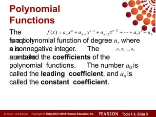
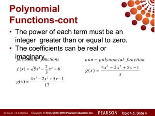
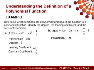
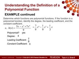
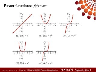
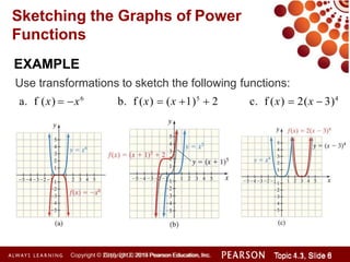
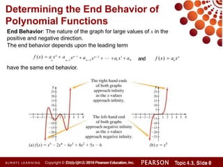
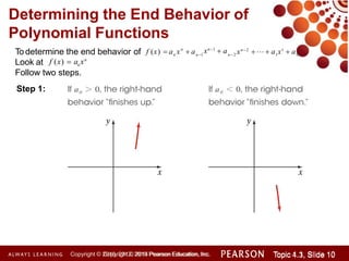
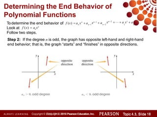
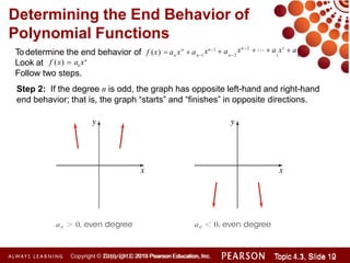
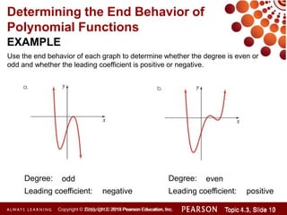
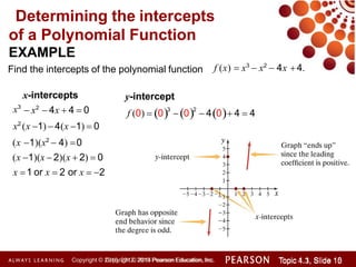
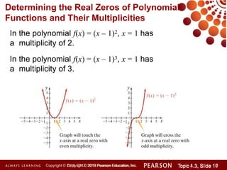
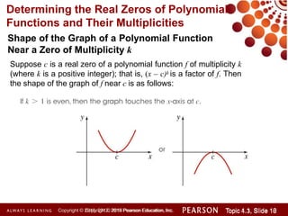
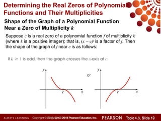
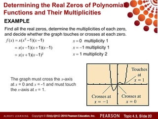
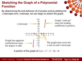
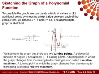
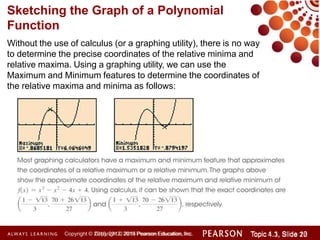
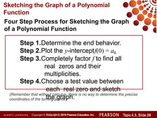
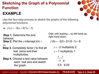
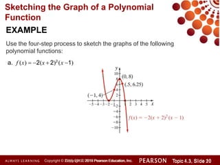
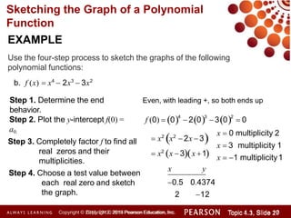
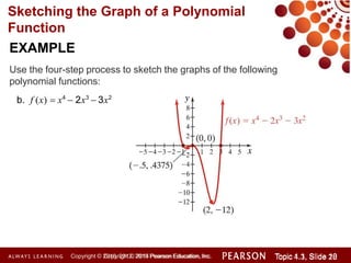
Topic 4.3
The Graphs of
Polynomial
Functions
Copyright © 2014 Pearson Education, Inc. Topic 1.1, Slide 1
Topic 4.3, Slide 1
Copyright © 2010, 2012, 2015 Pearson Education, Inc.

OBJECTIVES
Topic 4.3, Slide 2
1. Understanding the Definition of a Polynomial Function
2. Sketching the Graphs of Power Functions
3. Determining the End Behavior of Polynomial Functions
4. Determining the Intercepts of a Polynomial Function
5. Determining the Real Zeros of Polynomial Functions
and Their Multiplicities
6. Sketching the Graph of a Polynomial Function
7. Determining a Possible Equation of a Polynomial
Function Giving Its Graph

Polynomial
Functions
Topic 4.3, Slide 3
The
function
is a polynomial function of degree n, where
n is
a nonnegative integer. The
numbers
are called the coefficients of the
polynomial functions. The number a0 is
called the leading coefficient, and an is
called the constant coefficient.
0
n
f (x)  a x  a xn2
xn1
 a    a x1
 a
n n1 n2 1
a1,a2, ...,an

Polynomial
Functions-cont
• The power of each term must be an
integer greater than or equal to zero.
• The coefficients can be real or
imaginary.
17
4x3
 2x2
 5x 1
g(x) 
3
f (x)  5x4

2
x2
 6
polynomial functions
x
Topic 4.3, Slide 4
4x3
 2x2
 5x 1
g(x) 
non  polynomial function

Understanding the Definition of a
Polynomial Function
a. f (x)  3x3
 2x2

Polynomial? yes
1
6
EXAMPLE
Determine which functions are polynomial functions. If the function is a
polynomial function, identify the degree, the leading coefficient, and the
constant coefficient.
Degree:
Leading Coefficient:
3
3
Constant Coefficient: 
1
6
5 3 2
Topic 4.3, Slide 5
7
b. g(x)  4x  3x  x   3
x
Polynomial? no

Understanding the Definition of a
Polynomial Function
3x  x2
7x4
c. h(x) 
EXAMPLE continued
Determine which functions are polynomial functions. If the function is a
polynomial function, identify the degree, the leading coefficient, and the
constant coefficient.
Degree:
9
Polynomial? yes
4
Constant Coefficient:
Leading Coefficient:
7
9
0

7
x4

1
x2

1
x
9 9 3
Topic 4.3, Slide 6

Power functions: f(x) = axn
Topic 4.3, Slide 7

Sketching the Graphs of Power
Functions
EXAMPLE
Use transformations to sketch the following functions:
a. f (x)  x6
b. f (x)  (x 1)5
 2 c. f (x)  2(x  3)4
Topic 4.3, Slide 8

Determining the End Behavior of
Polynomial Functions
End Behavior: The nature of the graph for large values of x in the
positive and negative direction.
The end behavior depends upon the leading term
1 0
n2
xn1
 a
f (x)  a xn
 a
n n1 n
xn2
  a x1
 a f (x)  a xn
and
have the same end behavior.
Topic 4.3, Slide 9

To determine the end behavior of
Look at
0
1
n
n
f (x)  a x  a xn2
   a x1
 a
n2
xn1
 a
n1
n
f (x)  a xn
Follow two steps.
Step 1:
Topic 4.3, Slide 10

Look at
n
f (x)  a x  a xn2
   a x1
 a
1 0
xn1
 a
n n1 n2
n
f (x)  a xn
Follow two steps.
Step 2: If the degree n is odd, the graph has opposite left-hand and right-hand
end behavior; that is, the graph “starts” and “finishes” in opposite directions.
Topic 4.3, Slide 11

Look at
n
f (x)  a x  a xn2
   a x1
 a
1 0
xn1
 a
n n1 n2
n
f (x)  a xn
Follow two steps.
Step 2: If the degree n is odd, the graph has opposite left-hand and right-hand
end behavior; that is, the graph “starts” and “finishes” in opposite directions.
Topic 4.3, Slide 12

EXAMPLE
Use the end behavior of each graph to determine whether the degree is even or
odd and whether the leading coefficient is positive or negative.
Degree: odd
Leading coefficient: negative
Topic 4.3, Slide 13
Degree: even
Leading coefficient: positive

Determining the intercepts
of a Polynomial Function
• y-intercept: Found by evaluating
f(0)
• x-intercepts:Found by solving f(x) =
0
Topic 4.3, Slide 14

Determining the intercepts
EXAMPLE
Find the intercepts of the polynomial function f (x)  x3
 x2
 4x 4.
x3
x2
(x 1) 4(x 1)  0
(x 1)(x2
 4) 0
(x 1)(x  2)(x  2)  0
x 1 or x  2 or x  2
x-intercepts
 x2
 4x  4  0
y-intercept
f (0)  03
02
 40 4  4
Topic 4.3, Slide 15

Determining the Real Zeros of Polynomial
Functions and Their Multiplicities
Topic 4.3, Slide 16
If (x – c) is a factor of a polynomial function, then
x = c is a zero.
If f is a polynomial function and x = c is a zero,
then (x – c) is a factor.
If a factor (x – c) occurs n times in a polynomial, n
is an integer greater than 0, the zero x = c is said
to have a multiplicity n.

In the polynomial f(x) = (x – 1)2, x = 1 has
a multiplicity of 2.
In the polynomial f(x) = (x – 1)3, x = 1 has
a multiplicity of 3.
Topic 4.3, Slide 17

Shape of the Graph of a Polynomial Function
Near a Zero of Multiplicity k
Suppose c is a real zero of a polynomial function f of multiplicity k
(where k is a positive integer); that is, (x – c)k is a factor of f. Then
the shape of the graph of f near c is as follows:
Topic 4.3, Slide 18

Shape of the Graph of a Polynomial Function
Near a Zero of Multiplicity k
Suppose c is a real zero of a polynomial function f of multiplicity k
(where k is a positive integer); that is, (x – c)k is a factor of f. Then
the shape of the graph of f near c is as follows:
Topic 4.3, Slide 19

EXAMPLE
Find all the real zeros, determine the multiplicities of each zero,
and decide whether the graph touches or crosses at each zero.
f (x)  x(x2
1)(x 1)
 x(x 1)(x 1)(x1)
 x(x 1)(x 1)2
x  0 multiplicity 1
x  1 multiplicity 1
The graph must cross the x-axis
at x = 0 and x = -1 and must touch
the x-axis at x = 1.
Topic 4.3, Slide 20

By determining the end behavior of a function and by plotting the
x-intercepts and y-intercept, we can begin to sketch the graph.
Sketching the Graph of a Polynomial
Function
A portion of the graph of f (x)  x3
 x2
 4x  4
Topic 4.3, Slide 21

To complete the graph, we can create a table of values to plot
additional points by choosing a test value between each of the
zeros. Here, we choose x = -1 and x = 1.5. The approximate
graph is sketched.
Function
We see from the graph that there are two turning points. A polynomial
function of degree n has at most n - 1 turning points. A turning point in which
the graph changes from increasing to decreasing is also called a relative
maximum. A turning point in which the graph changes from decreasing to
increasing is called a relative minimum.
Topic 4.3, Slide 22

Without the use of calculus (or a graphing utility), there is no way
to determine the precise coordinates of the relative minima and
relative maxima. Using a graphing utility, we can use the
Maximum and Minimum features to determine the coordinates of
the relative maxima and minima as follows:
Function
Topic 4.3, Slide 23

Four Step Process for Sketching the Graph
Step 1.Determine the end behavior.
Step 2.Plot the y-interceptf(0) = a0.
Step 3.Completely factor f to find all
real zeros and their
multiplicities.
Step 4.Choose a test value between
each real zero and sketch
the graph.
Function
(Remember that without calculus, there is no way to determine the precise
coordinates of the turning points.)
Topic 4.3, Slide 24

EXAMPLE
Use the four-step process to sketch the graphs of the following
polynomial functions:
a. f (x)  2(x  2)2
(x 1)
Function
Step 1. Determine the end
behavior.
Step 2. Plot the y-intercept f(0) =
a0.
Step 3. Completely factor f to find all
multiplicities.
Step 4. Choose a test value between
the graph.
Odd, with leading -, so left hand up,
right hand down.
f (0)  2(0 2)2
(0 1)  8
x  2 multiplicity 2
x y
0.5 6.25
Topic 4.3, Slide 25
1 4

EXAMPLE
a. f (x)  2(x  2)2
(x 1)
Function
Topic 4.3, Slide 26

EXAMPLE
b. f (x)  x4
 2x3
 3x2
Function
Step 1. Determine the end
behavior.
Step 2. Plot the y-intercept f(0) =
a0.
Step 3. Completely factor f to find all
multiplicities.
Step 4. Choose a test value between
the graph.
Even, with leading +, so both ends up
x  1 multiplicity1
0.5 0.4374
2 12
Topic 4.3, Slide 27
x y
 x2
x2
 2x 3
 x2
x 3x 1
f (0)  04
 203
302
 0

EXAMPLE
b. f (x)  x4
 2x3
 3x2
Function
Topic 4.3, Slide 28

Determining a Possible Equation of a
Polynomial Function Given its Graph
EXAMPLE
Analyze the graph to address the following about the
polynomial function it represents
a.Is the degree of the polynomial
function even or odd?
Odd because the graph starts up
and finishes down.
b. Is the leading coefficient positive or negative?
Negative because the right hand behavior finishes down
Topic 4.3, Slide 29

of each.
EXAMPLE continued
c. What is the value of the constant coefficient?
2 because the y-intercept is 2.
d. Identify the real zeros, and state the multiplicity
x =-5 multiplicity odd
x =-2 multiplicity odd
x =1 multiplicity even
x =4 multiplicity odd
Topic 4.3, Slide 30

EXAMPLE continued
e. Select from this list a possible function that
could be represented by this graph.
ii. f (x) 
20
1
i. f (x)  
1
(x  5)(x  2)(x 1)2
(x  4)
800
(x  5)2
(x  2)2
(x 1)(x  4)2
20
iii. f (x) 
1
(x  5)(x  2)(x 1)2
(x  4)
10
iv. f (x)  
1
(x  5)(x  2)(x 1)2
(x  4)
Topic 4.3, Slide 31

end behavior.....pptx

More Related Content

What's hot

Similar to end behavior.....pptx

More from LunaLedezma3

Recently uploaded

end behavior.....pptx