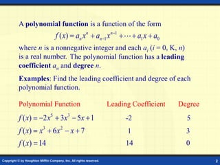
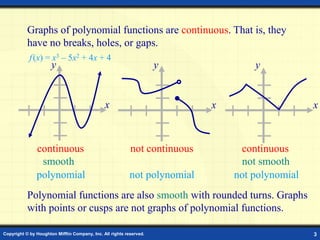
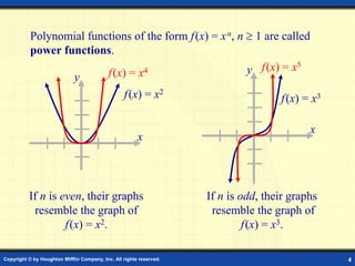
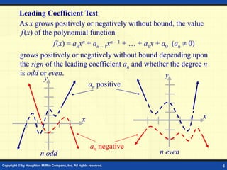
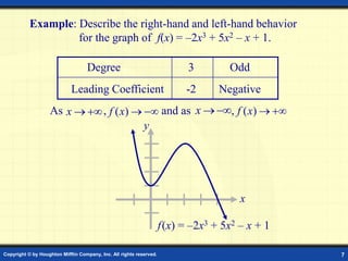
This document discusses graphs of polynomial functions. It defines a polynomial function as a function of the form f(x) = anxn + an-1xn-1 + ... + a1x + a0, where n is a nonnegative integer and each ai is a real number. The degree of the polynomial is n and the leading coefficient is an. Polynomial graphs are continuous and smooth without breaks or cusps. The behavior of graphs as x approaches positive or negative infinity depends on the sign of the leading coefficient and whether the degree is odd or even. Polynomials can have real zeros where they intersect the x-axis. Their graphs may have up to n turning points and n zeros.

1. Graphs of Polynomial
Functions
Digital Lesson

2. Copyright © by Houghton Mifflin Company, Inc. All rights reserved. 2
A polynomial function is a function of the form
1
1 1 0
( ) n n
n n
f x a x a x a x a


    
where n is a nonnegative integer and each ai (i = 0, , n)
is a real number. The polynomial function has a leading
coefficient an and degree n.
Examples: Find the leading coefficient and degree of each
polynomial function.
Polynomial Function Leading Coefficient Degree
5 3
( ) 2 3 5 1
f x x x x
    
3 2
( ) 6 7
f x x x x
   
( ) 14
f x 
-2 5
1 3
14 0

3. Copyright © by Houghton Mifflin Company, Inc. All rights reserved. 3
Graphs of polynomial functions are continuous. That is, they
have no breaks, holes, or gaps.
Polynomial functions are also smooth with rounded turns. Graphs
with points or cusps are not graphs of polynomial functions.
x
y
x
y
continuous not continuous continuous
smooth not smooth
polynomial not polynomial not polynomial
x
y
f(x) = x3 – 5x2 + 4x + 4

4. Copyright © by Houghton Mifflin Company, Inc. All rights reserved. 4
Polynomial functions of the form f(x) = xn, n  1 are called
power functions.
If n is even, their graphs
resemble the graph of
f(x) = x2.
If n is odd, their graphs
resemble the graph of
f(x) = x3.
x
y
x
y
f(x) = x2
f(x) = x5
f(x) = x4
f(x) = x3

5. Copyright © by Houghton Mifflin Company, Inc. All rights reserved. 5
Example: Sketch the graph of f(x) = –(x + 2)4 .
This is a shift of the graph of y = –x4 two units to the left.
This, in turn, is the reflection of the graph of y = x4 in the x-axis.
x
y
y = x4
y = –x4
f(x) = –(x + 2)4

6. Copyright © by Houghton Mifflin Company, Inc. All rights reserved. 6
Leading Coefficient Test
As x grows positively or negatively without bound, the value
f(x) of the polynomial function
f(x) = anxn + an – 1xn – 1 + … + a1x + a0 (an  0)
grows positively or negatively without bound depending upon
the sign of the leading coefficient an and whether the degree n
is odd or even.
x
y
x
y
n odd n even
an positive
an negative

7. Copyright © by Houghton Mifflin Company, Inc. All rights reserved. 7
Example: Describe the right-hand and left-hand behavior
for the graph of f(x) = –2x3 + 5x2 – x + 1.
As , and as ,


x


x 

)
(x
f


)
(x
f
Negative
-2
Leading Coefficient
Odd
3
Degree
x
y
f(x) = –2x3 + 5x2 – x + 1

8. Copyright © by Houghton Mifflin Company, Inc. All rights reserved. 8
A real number a is a zero of a function y = f(x)
if and only if f(a) = 0.
A turning point of a graph of a function is a point at which the
graph changes from increasing to decreasing or vice versa.
A polynomial function of degree n has at most n – 1 turning
points and at most n zeros.
Real Zeros of Polynomial Functions
If y = f(x) is a polynomial function and a is a real number then
the following statements are equivalent.
1. a is a zero of f.
2. a is a solution of the polynomial equation f(x) = 0.
3. x – a is a factor of the polynomial f(x).
4. (a, 0) is an x-intercept of the graph of y = f(x).

9. Copyright © by Houghton Mifflin Company, Inc. All rights reserved. 9
Example: Find all the real zeros and turning points of the graph
of f(x) = x4 – x3 – 2x2.
Factor completely: f(x) = x4 – x3 – 2x2 = x2(x + 1)(x – 2).
The real zeros are x = –1, x = 0, and x = 2.
These correspond to the
x-intercepts (–1, 0), (0, 0) and (2, 0).
The graph shows that
there are three turning points.
Since the degree is four, this is
the maximum number possible.
y
x
f(x) = x4 – x3 – 2x2
Turning point
Turning point
Turning
point

10. Copyright © by Houghton Mifflin Company, Inc. All rights reserved. 10
Example: Determine the multiplicity of the zeros
of f(x) = (x – 2)3(x +1)4.
Zero Multiplicity Behavior
2
–1
3
4
odd
even
crosses x-axis
at (2, 0)
touches x-axis
at (–1, 0)
Repeated Zeros
If k is the largest integer for which (x – a)k is a factor of f(x)
and k > 1, then a is a repeated zero of multiplicity k.
1. If k is odd the graph of f(x) crosses the x-axis at (a, 0).
2. If k is even the graph of f(x) touches, but does not cross
through, the x-axis at (a, 0).
x
y

11. Copyright © by Houghton Mifflin Company, Inc. All rights reserved. 11
Intermediate Value Theorem
• Let f be a polynomial function with real
coefficients. If f(a) and f(b) have opposite signs,
then there is at least one value c between a and b
for which f(c) = 0
3
and
2
between
zero
real
a
has
5
2
)
(
Show 3


 x
x
x
f

12. Copyright © by Houghton Mifflin Company, Inc. All rights reserved. 12
Example: Sketch the graph of f(x) = 4x2 – x4.
1. Write the polynomial function in standard form: f(x) = –x4 + 4x2
The leading coefficient is negative and the degree is even.
2. Find the zeros of the polynomial by factoring.
f(x) = –x4 + 4x2 = –x2(x2 – 4) = – x2(x + 2)(x –2)
Zeros:
x = –2, 2 multiplicity 1
x = 0 multiplicity 2
x-intercepts:
(–2, 0), (2, 0) crosses through
(0, 0) touches only
Example continued
as , 

)
(x
f


x
x
y
(2, 0)
(0, 0)
(–2, 0)

13. Copyright © by Houghton Mifflin Company, Inc. All rights reserved. 13
Example continued: Sketch the graph of f(x) = 4x2 – x4.
3. Since f(–x) = 4(–x)2 – (–x)4 = 4x2 – x4 = f(x), the graph is
symmetrical about the y-axis.
4. Plot additional points and their reflections in the y-axis:
(1.5, 3.9) and (–1.5, 3.9 ), (0.5, 0.94 ) and (–0.5, 0.94)
5. Draw the graph.
x
y
(1.5, 3.9)
(–1.5, 3.9 )
(–0.5, 0.94 ) (0.5, 0.94)