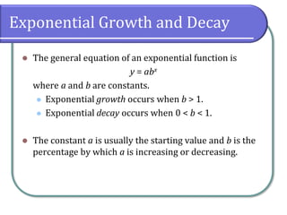
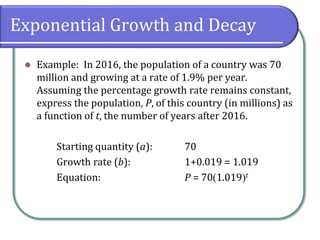
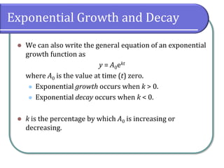
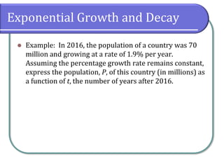
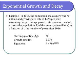
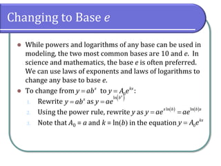
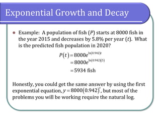
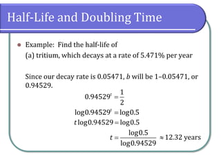
* Model exponential growth and decay
* Use Newton's Law of Cooling
* Use logistic-growth models
* Choose an appropriate model for data
* Express an exponential model in base e
2. Concepts and Objectives
⚫ Objectives for this section are
⚫ Model exponential growth and decay.
⚫ Use Newton’s Law of Cooling.
⚫ Use logistic-growth models.
⚫ Choose an appropriate model for data.
⚫ Express an exponential model in base e.
3. Exponential Growth and Decay
⚫ The general equation of an exponential function is
y = abx
where a and b are constants.
⚫ Exponential growth occurs when b > 1.
⚫ Exponential decay occurs when 0 < b < 1.
⚫ The constant a is usually the starting value and b is the
percentage by which a is increasing or decreasing.
4. Exponential Growth and Decay
⚫ Example: In 2016, the population of a country was 70
million and growing at a rate of 1.9% per year.
Assuming the percentage growth rate remains constant,
express the population, P, of this country (in millions) as
a function of t, the number of years after 2016.
5. Exponential Growth and Decay
⚫ Example: In 2016, the population of a country was 70
million and growing at a rate of 1.9% per year.
Assuming the percentage growth rate remains constant,
express the population, P, of this country (in millions) as
a function of t, the number of years after 2016.
Starting quantity (a): 70
Growth rate (b): 1+0.019 = 1.019
Equation: P = 70(1.019)t
6. Exponential Growth and Decay
⚫ We can also write the general equation of an exponential
growth function as
y = A0ekt
where A0 is the value at time (t) zero.
⚫ Exponential growth occurs when k > 0.
⚫ Exponential decay occurs when k < 0.
⚫ k is the percentage by which A0 is increasing or
decreasing.
7. Exponential Growth and Decay
⚫ Example: In 2016, the population of a country was 70
million and growing at a rate of 1.9% per year.
Assuming the percentage growth rate remains constant,
express the population, P, of this country (in millions) as
a function of t, the number of years after 2016.
8. Exponential Growth and Decay
⚫ Example: In 2016, the population of a country was 70
million and growing at a rate of 1.9% per year.
Assuming the percentage growth rate remains constant,
express the population, P, of this country (in millions) as
a function of t, the number of years after 2016.
Starting quantity (A0): 70
Growth rate (k): 0.019
Equation: P = 70e0.019t
9. Exponential Growth and Decay
⚫ Example: A population of fish (P) starts at 8000 fish in
the year 2015 and decreases by 5.8% per year (t). What
is the predicted fish population in 2020?
10. Changing to Base e
⚫ While powers and logarithms of any base can be used in
modeling, the two most common bases are 10 and e. In
science and mathematics, the base e is often preferred.
We can use laws of exponents and laws of logarithms to
change any base to base e.
⚫ To change from to :
1. Rewrite as
2. Using the power rule, rewrite y as
3. Note that A0 = a and k = ln(b) in the equation
x
y ab
= 0
kx
y A e
=
x
y ab
=
( )
ln x
b
y ae
=
( ) ( )
ln ln
x b b x
y ae ae
= =
0
kx
y A e
=
11. Changing to Base e
⚫ Example: Change the function to base e.
( )
2.5 3.1
x
y =
12. Changing to Base e
⚫ Example: Change the function to base e.
( )
2.5 3.1
x
y =
( )
( )
( )
ln 3.1
ln 3.1
2.5 3.1
2.5
2.5
x
x
x
y
e
e
=
=
=
13. Exponential Growth and Decay
⚫ Example: A population of fish (P) starts at 8000 fish in
the year 2015 and decreases by 5.8% per year (t). What
is the predicted fish population in 2020?
14. Exponential Growth and Decay
⚫ Example: A population of fish (P) starts at 8000 fish in
the year 2015 and decreases by 5.8% per year (t). What
is the predicted fish population in 2020?
We first need to write this as an exponential equation:
(because the population is decreasing, we have to use a
decay model)
Now, we convert this to an exponential decay function:
( ) ( )
8000 1 0.058 8000 0.942
t t
y = − =
( ) ( )
ln 0.942
8000
t
P t e
=
15. Exponential Growth and Decay
⚫ Example: A population of fish (P) starts at 8000 fish in
the year 2015 and decreases by 5.8% per year (t). What
is the predicted fish population in 2020?
Honestly, you could get the same answer by using the first
exponential equation, , but most of the
problems you will be working require the natural log.
( ) ( )
ln 0.942
8000
t
P t e
=
( )( )
ln 0.942 5
8000
5934 fish
e
=
=
( )
8000 0.942
t
y =
16. Half-Life and Doubling Time
⚫ Half-life refers to the length of time it takes for an
exponential decay to reach half of its starting quantity.
⚫ Doubling time refers to the length of time it takes for an
exponential growth to reach double its starting quantity.
⚫ Both of these problems are actually worked the same
way. To find the half-life (or doubling time), let the initial
quantity be 1 and set the equation equal to ½ (or 2) and
solve for t. Whether you use the common log (base-10)
or the natural log (base e) is mostly a matter of taste and
convenience. Most of the time, you can work the
problems using either.
17. Half-Life and Doubling Time
⚫ Example: Find the half-life of
(a) tritium, which decays at a rate of 5.471% per year
(b) a radioactive substance which decays at a rate of
11% per minute.
18. Half-Life and Doubling Time
⚫ Example: Find the half-life of
(a) tritium, which decays at a rate of 5.471% per year
Since our decay rate is 0.05471, b will be 1–0.05471, or
0.94529.
=
1
0.94529
2
t
=
log0.94529 log0.5
t
=
log0.94529 log0.5
t
=
log0.5
log0.94529
t 12.32 years
19. Half-Life and Doubling Time
⚫ Example: Find the half-life of
(a) tritium, which decays at a rate of 5.471% per year
You could also use ln instead of log and work the
problem the same way. That being said, sometimes you
may want to find the continuous decay rate to use in an
exponential function, .
( ) 0
kt
A t A e
=
( ) ( )
( )
ln 0.94529
0
0.05626
0
t
t
A t A e
A t A e−
=
=
20. Half-Life and Doubling Time
⚫ Example: Find the half-life of
(b) a radioactive substance which decays at a continuous
rate of 11% per minute.
Since this is continuous decay, we use the natural log:
−
=
0.11 1
2
t
e
−
=
0.11
ln ln0.5
t
e
− =
0.11 ln0.5
t
=
−
ln0.5
0.11
t 6.30 minutes
21. Half-Life and Doubling Time
⚫ Example: A colony of bacteria has a growth rate of
4.97% per hour. How long until the colony has doubled
in size?
22. Half-Life and Doubling Time
⚫ Example: A colony of bacteria has a growth rate of
4.97% per hour. How long until the colony has doubled
in size?
( )
( )
( )
( )
1 0.0497 2
1.0497 2
ln 1.0497 ln2
ln2
14.29 hours
ln 1.0497
t
t
t
t
+ =
=
=
= =
23. Carbon-14 Dating
⚫ Carbon-14 is a radioactive isotope of carbon that has a
half-life of 5,730 years, and it occurs in small quantities
in the carbon dioxide in our atmosphere. Most of the
carbon on Earth is carbon-12, and the ratio of carbon-14
to carbon-12 in the atmosphere has been calculated for
the last 60,000 years.
⚫ As long as a plant or animal is alive, the ratio of the two
isotopes in its body is close to the ratio in the
atmosphere. When it dies, the carbon-14 in its body
decays and is not replaced. By comparing the ratio of
carbon-14 to carbon-12, the date the plant or animal
died can be approximated.
24. Carbon-14 Dating (cont.)
⚫ Since the half-life of carbon-14 is 5,730 years, the
formula for the amount of carbon-14 remaining after t
years is
⚫ To find the age of an object, we solve this equation for t:
where r is the ratio of A to A0.
( )
ln 0.5
5730
0
0.000121
0
or
t
t
A A e
A A e−
( )
ln
0.000121
r
t =
−
25. Carbon-14 Dating (cont.)
⚫ Example: A bone fragment is found that contains 20% of
its original carbon-14. To the nearest year, how old is
the bone?
26. Carbon-14 Dating (cont.)
⚫ Example: A bone fragment is found that contains 20% of
its original carbon-14. To the nearest year, how old is
the bone?
⚫ You don’t necessarily have to memorize this formula
because you can always use the general form to derive
this.
( )
ln 0.20
0.000121
13,301 years
t =
−
27. Newton’s Law of Cooling
⚫ When a hot object is left in surrounding air that is at a
lower temperature, the object’s temperature will
decrease exponentially, leveling off as it approaches the
surrounding air temperature.
⚫ The temperature of an object, T, in surrounding air with
temperature Ts will behave according to the formula
where t is time, A is the difference between the initial
temperature of the object and the surrounding air, and k
is a constant, the continuous rate of cooling of the object.
( ) kt
s
T t Ae T
= +
28. Newton’s Law of Cooling (cont.)
⚫ Example: A cheesecake is taken out of the oven with an
ideal internal temperature of 165F, and is placed into a
35F refrigerator. After 10 minutes, the cheesecake has
cooled to 150F. If we must wait until the cheesecake
has cooled to 70F before we eat it, how long will we
have to wait?
29. Newton’s Law of Cooling (cont.)
⚫ Solution: Because the surrounding air temperature in
the refrigerator is 35, the cheesecake’s temperature will
decay exponentially toward 35, following the equation
⚫ The initial temperature was 165, so T(0) = 165.
⚫ We were given another data point, T(10) = 150, which
we can use to solve for k.
( ) 35
kt
T t Ae
= +
0
165 35
130
k
Ae
A
= +
=
30. Newton’s Law of Cooling (cont.)
⚫ Solution (cont.):
( )
10
10
10
150 130 35
115 130
115
130
115
ln 10
130
115
ln
130
0.0123
10
k
k
k
e
e
e
k
k
= +
=
=
=
= −
31. Newton’s Law of Cooling (cont.)
⚫ Solution (cont.): All of this gives us the equation for the
cooling of the cheesecake:
⚫ Now we can solve for the time it will take for the
temperature to reach 70:
( ) 0.0123
130 35
t
T t e−
= +
32. Newton’s Law of Cooling (cont.)
⚫ Solution (cont.): Now we can solve for the time it will
take for the temperature to reach 70:
or about 1 hour and 47 minutes.
0.0123
0.0123
70 130 35
35 130
35
ln 0.0123
130
35
ln
130
106.68 minutes
0.0123
t
t
e
e
t
t
−
−
= +
=
= −
=
−
33. Logistic Growth Models
⚫ Exponential growth rarely continues forever.
Exponential models, while useful in the short term, tend
to fall apart the longer they continue.
⚫ Consider someone who saves a penny on day one and
resolves to double that amount every day. By the end of
the second week, he would be trying to save $163.84 in
one day. By the end of the month, he would be trying to
save $10,737,418.24!
⚫ Eventually, an exponential model must begin to reach
some limiting value, and then the growth is forced to
slow. The model is called the logistic growth model.
34. Logistic Growth Models (cont.)
⚫ The logistic growth model is approximately exponential
at first, but it has a reduced rate of growth as the output
approaches the model’s upper bound, called the
carrying capacity. For constants a, b, and c, the
logistice growth of a population over time t is
represented by the model
( )
1 bt
c
f t
ae−
=
+
35. Logistic Growth Models (cont.)
⚫ An influenza epidemic spreads through a population
rapidly, at a rate that depends on two factors: The more
people who have the flu, the more rapidly it spreads, and
also the more uninfected people there are, the more
rapidly it spreads. These two factors make the logistic
model a good one to study the spread of communicable
diseases. And, clearly, there is a maximum value for the
number of people infected: the entire population.
36. Logistic Growth Models (cont.)
⚫ Example: At time t = 0, there is one person in a
community of 1,000 people who has the flu. So in that
community, at most 1,000 people can have the flu.
Researchers find that for this particular strain of the flu,
the logistic growth constant is b = 0.6030. Estimate the
number of people in this community who will have this
flu after ten days.
37. Logistic Growth Models (cont.)
⚫ Example: At time t = 0, there is one person in a
community of 1,000 people who has the flu. So in that
community, at most 1,000 people can have the flu.
Researchers find that for this particular strain of the flu,
the logistic growth constant is b = 0.6030. Estimate the
number of people in this community who will have this
flu after ten days.
⚫ Solution: We substitute the given data into the logistic
growth model:
( ) 0.6030
1000
1 t
f t
ae−
=
+
38. Logistic Growth Models (cont.)
⚫ Solution (cont.): To find a, we use the formula that the
number of cases at time t = 0 is 1, from which it follows
that
and after 10 days,
( )
1000
0 1
1
999
f
a
a
= =
+
=
( ) ( )
0.6030 10
1000
10 294 people
1 999
f
e
−
=
+