The document summarizes different types of derivatives:
Simple derivatives involve a single input and output. Implicit derivatives are taken for equations with two or more variables, treating one as the independent variable. An example finds derivatives of u with respect to v and v with respect to u for the equation 2u^2 - v^3 = 2 - uv. The derivatives are related by the reciprocal relationship in differential notation.
![Summary of Derivatives
In this section we summarize the various types of
derivatives we have encountered and the algebra
associated with each type.
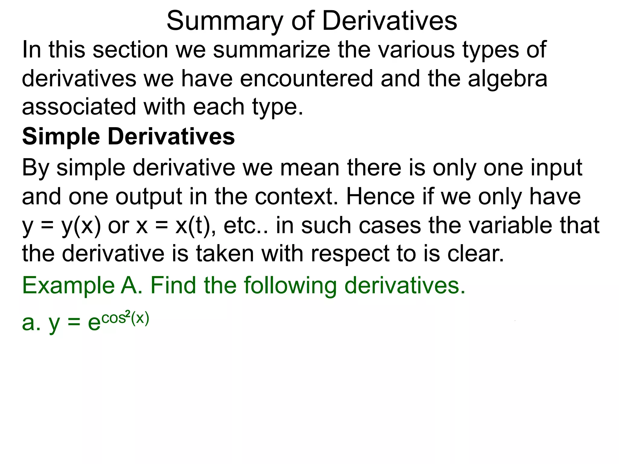
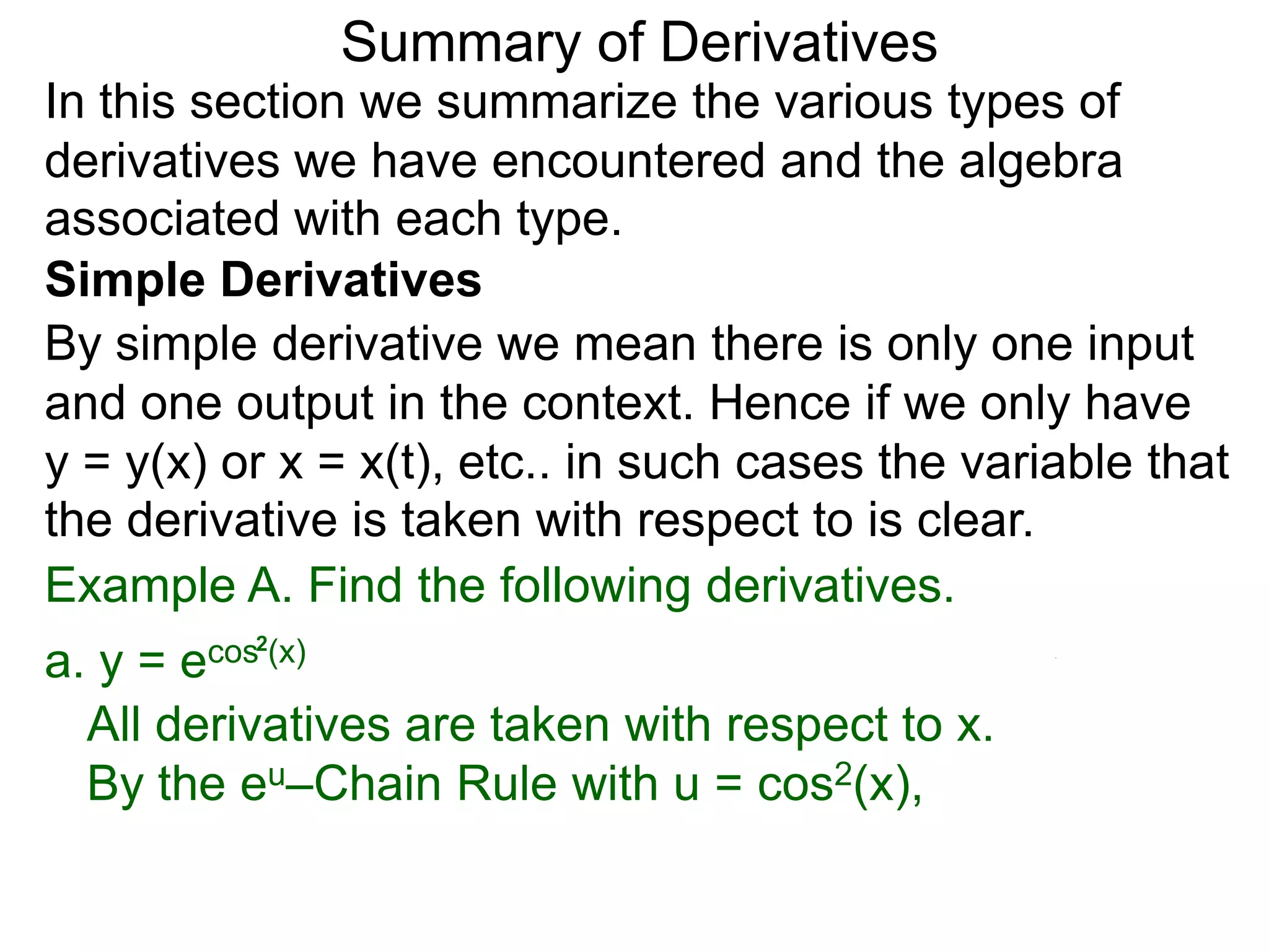
Simple Derivatives
By simple derivative we mean there is only one input
and one output in the context. Hence if we only have
y = y(x) or x = x(t), etc.. in such cases the variable that
the derivative is taken with respect to is clear.
Example A. Find the following derivatives.
a. y =e cos2(x)
All derivatives are taken with respect to x.
By the eu–Chain Rule with u = cos2(x),
y' = e cos2(x) [cos2(x)]'](https://image.slidesharecdn.com/4-4reviewonderivatives-120430211412-phpapp02/75/4-4-review-on-derivatives-8-2048.jpg)
![Summary of Derivatives
In this section we summarize the various types of
derivatives we have encountered and the algebra
associated with each type.
Simple Derivatives
By simple derivative we mean there is only one input
and one output in the context. Hence if we only have
y = y(x) or x = x(t), etc.. in such cases the variable that
the derivative is taken with respect to is clear.
Example A. Find the following derivatives.
a. y =e cos2(x)
All derivatives are taken with respect to x.
By the eu–Chain Rule with u = cos2(x),
y' = e cos2(x) [cos2(x)]' by the Power Chain Rule
2
=e cos2 (x)2cos(x)[cos(x)]'](https://image.slidesharecdn.com/4-4reviewonderivatives-120430211412-phpapp02/75/4-4-review-on-derivatives-9-2048.jpg)
![Summary of Derivatives
In this section we summarize the various types of
derivatives we have encountered and the algebra
associated with each type.
Simple Derivatives
By simple derivative we mean there is only one input
and one output in the context. Hence if we only have
y = y(x) or x = x(t), etc.. in such cases the variable that
the derivative is taken with respect to is clear.
Example A. Find the following derivatives.
a. y =e cos2(x)
All derivatives are taken with respect to x.
By the eu–Chain Rule with u = cos2(x),
y' = e cos2(x) [cos2(x)]' by the Power Chain Rule
=e cos2 (x)2cos(x)[cos(x)]' = –2ecos2 (x)cos(x)sin(x)](https://image.slidesharecdn.com/4-4reviewonderivatives-120430211412-phpapp02/75/4-4-review-on-derivatives-10-2048.jpg)
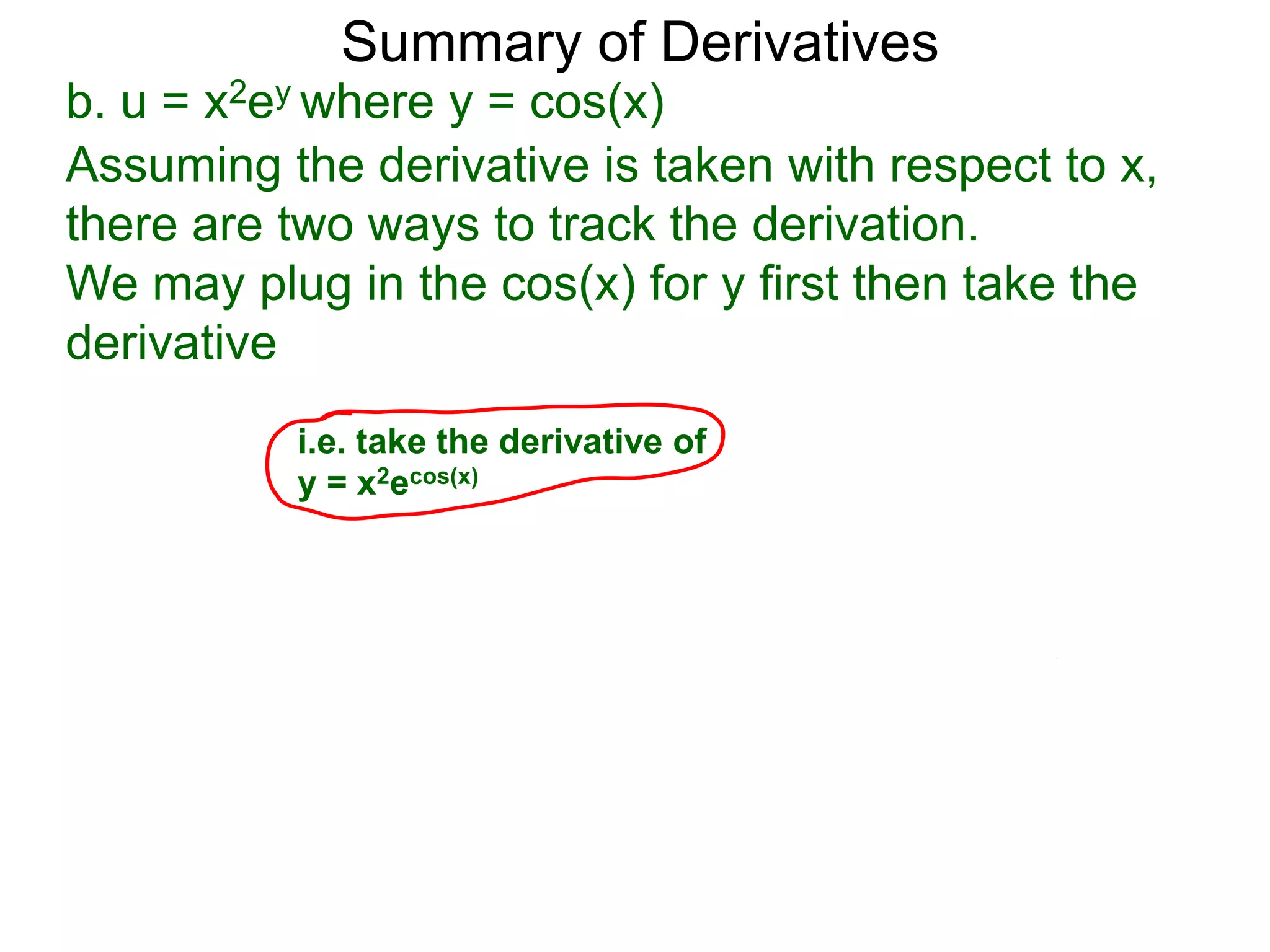
![Summary of Derivatives
b. u = x2ey where y = cos(x)
Assuming the derivative is taken with respect to x,
there are two ways to track the derivation.
We may plug in the cos(x) for y first then take the
derivative or as we would proceed with the
Product Rule and track the derivation with y.
u' = [x2]'ey + x2[ey]'](https://image.slidesharecdn.com/4-4reviewonderivatives-120430211412-phpapp02/75/4-4-review-on-derivatives-16-2048.jpg)
![Summary of Derivatives
b. u = x2ey where y = cos(x)
Assuming the derivative is taken with respect to x,
there are two ways to track the derivation.
We may plug in the cos(x) for y first then take the
derivative or as we would proceed with the
Product Rule and track the derivation with y.
u' = [x2]'ey + x2[ey]'
= 2xey + x2ey[y]'](https://image.slidesharecdn.com/4-4reviewonderivatives-120430211412-phpapp02/75/4-4-review-on-derivatives-17-2048.jpg)
![Summary of Derivatives
b. u = x2ey where y = cos(x)
Assuming the derivative is taken with respect to x,
there are two ways to track the derivation.
We may plug in the cos(x) for y first then take the
derivative or as we would proceed with the
Product Rule and track the derivation with y.
u' = [x2]'ey + x2[ey]'
= 2xey + x2ey[y]'
Substitute y = cos(x) and y' = –sin(x), we have
u' = 2xecos(x) – x2sin(x)ecos(x)](https://image.slidesharecdn.com/4-4reviewonderivatives-120430211412-phpapp02/75/4-4-review-on-derivatives-18-2048.jpg)
![Summary of Derivatives
b. u = x2ey where y = cos(x)
Assuming the derivative is taken with respect to x,
there are two ways to track the derivation.
We may plug in the cos(x) for y first then take the
derivative or as we would proceed with the
Product Rule and track the derivation with y.
u' = [x2]'ey + x2[ey]'
= 2xey + x2ey[y]'
Substitute y = cos(x) and y' = –sin(x), we have
u' = 2xecos(x) – x2sin(x)ecos(x)
= xecos(x)(2 – xsin(x))](https://image.slidesharecdn.com/4-4reviewonderivatives-120430211412-phpapp02/75/4-4-review-on-derivatives-19-2048.jpg)
![Summary of Derivatives
b. u = x2ey where y = cos(x)
Assuming the derivative is taken with respect to x,
there are two ways to track the derivation.
We may plug in the cos(x) for y first then take the
derivative or as we would proceed with the
Product Rule and track the derivation with y.
u' = [x2]'ey + x2[ey]'
= 2xey + x2ey[y]'
Substitute y = cos(x) and y' = –sin(x), we have
u' = 2xecos(x) – x2sin(x)ecos(x)
= xecos(x)(2 – xsin(x))
The above derivation leads to implicit differentiation.](https://image.slidesharecdn.com/4-4reviewonderivatives-120430211412-phpapp02/75/4-4-review-on-derivatives-20-2048.jpg)
![Summary of Derivatives
Implicit Derivatives
In implicit differentiation, a two (or more)–variable
equation is given, we assume one of them as the
independent variable, say v, and we are to find the
derivative of the other variable with respect to v,
hence the Chain Rules are needed for derivatives of
the variable in the equations.
Example B. Given that 2u2 – v3 = 2 – uv,
a. Find the derivative of u with respect to v.
Taking the derivative with respect to v both sides,
[2u2 – v3 = 2 – uv]'](https://image.slidesharecdn.com/4-4reviewonderivatives-120430211412-phpapp02/75/4-4-review-on-derivatives-26-2048.jpg)
![Summary of Derivatives
Implicit Derivatives
In implicit differentiation, a two (or more)–variable
equation is given, we assume one of them as the
independent variable, say v, and we are to find the
derivative of the other variable with respect to v,
hence the Chain Rules are needed for derivatives of
the variable in the equations.
Example B. Given that 2u2 – v3 = 2 – uv,
a. Find the derivative of u with respect to v.
Taking the derivative with respect to v both sides,
[2u2 – v3 = 2 – uv]'
4uu' – 3v2 =](https://image.slidesharecdn.com/4-4reviewonderivatives-120430211412-phpapp02/75/4-4-review-on-derivatives-27-2048.jpg)
![Summary of Derivatives
Implicit Derivatives
In implicit differentiation, a two (or more)–variable
equation is given, we assume one of them as the
independent variable, say v, and we are to find the
derivative of the other variable with respect to v,
hence the Chain Rules are needed for derivatives of
the variable in the equations.
Example B. Given that 2u2 – v3 = 2 – uv,
a. Find the derivative of u with respect to v.
Taking the derivative with respect to v both sides,
[2u2 – v3 = 2 – uv]'
4uu' – 3v2 = –u'v – uv'](https://image.slidesharecdn.com/4-4reviewonderivatives-120430211412-phpapp02/75/4-4-review-on-derivatives-28-2048.jpg)
![Summary of Derivatives
Implicit Derivatives
In implicit differentiation, a two (or more)–variable
equation is given, we assume one of them as the
independent variable, say v, and we are to find the
derivative of the other variable with respect to v,
hence the Chain Rules are needed for derivatives of
the variable in the equations.
Example B. Given that 2u2 – v3 = 2 – uv,
a. Find the derivative of u with respect to v.
Taking the derivative with respect to v both sides,
[2u2 – v3 = 2 – uv]' 1
4uu' – 3v2 = –u'v – uv'](https://image.slidesharecdn.com/4-4reviewonderivatives-120430211412-phpapp02/75/4-4-review-on-derivatives-29-2048.jpg)
![Summary of Derivatives
Implicit Derivatives
In implicit differentiation, a two (or more)–variable
equation is given, we assume one of them as the
independent variable, say v, and we are to find the
derivative of the other variable with respect to v,
hence the Chain Rules are needed for derivatives of
the variable in the equations.
Example B. Given that 2u2 – v3 = 2 – uv,
a. Find the derivative of u with respect to v.
Taking the derivative with respect to v both sides,
[2u2 – v3 = 2 – uv]' 1
4uu' – 3v2 = –u'v – uv'
u'(4u + v) = 3v2 – u](https://image.slidesharecdn.com/4-4reviewonderivatives-120430211412-phpapp02/75/4-4-review-on-derivatives-30-2048.jpg)
![Summary of Derivatives
Implicit Derivatives
In implicit differentiation, a two (or more)–variable
equation is given, we assume one of them as the
independent variable, say v, and we are to find the
derivative of the other variable with respect to v,
hence the Chain Rules are needed for derivatives of
the variable in the equations.
Example B. Given that 2u2 – v3 = 2 – uv,
a. Find the derivative of u with respect to v.
Taking the derivative with respect to v both sides,
[2u2 – v3 = 2 – uv]' 1
4uu' – 3v2 = –u'v – uv'
u'(4u + v) = 3v2 – u
3v2 – u
so u' = 4u + v](https://image.slidesharecdn.com/4-4reviewonderivatives-120430211412-phpapp02/75/4-4-review-on-derivatives-31-2048.jpg)
![Summary of Derivatives
b. Find the derivative of v with respect to u.
Taking the derivative with respect to u both sides,
[2u2 – v3 = 2 – uv]'](https://image.slidesharecdn.com/4-4reviewonderivatives-120430211412-phpapp02/75/4-4-review-on-derivatives-33-2048.jpg)
![Summary of Derivatives
b. Find the derivative of v with respect to u.
Taking the derivative with respect to u both sides,
[2u2 – v3 = 2 – uv]'
4u – 3v2v' = –v – uv'](https://image.slidesharecdn.com/4-4reviewonderivatives-120430211412-phpapp02/75/4-4-review-on-derivatives-34-2048.jpg)
![Summary of Derivatives
b. Find the derivative of v with respect to u.
Taking the derivative with respect to u both sides,
[2u2 – v3 = 2 – uv]'
4u – 3v2v' = –v – uv'
uv' – 3v2v' = –v – 4u](https://image.slidesharecdn.com/4-4reviewonderivatives-120430211412-phpapp02/75/4-4-review-on-derivatives-35-2048.jpg)
![Summary of Derivatives
b. Find the derivative of v with respect to u.
Taking the derivative with respect to u both sides,
[2u2 – v3 = 2 – uv]'
4u – 3v2v' = –v – uv'
uv' – 3v2v' = –v – 4u
v'(u – 3v2) = – v – 4u so](https://image.slidesharecdn.com/4-4reviewonderivatives-120430211412-phpapp02/75/4-4-review-on-derivatives-36-2048.jpg)
![Summary of Derivatives
b. Find the derivative of v with respect to u.
Taking the derivative with respect to u both sides,
[2u2 – v3 = 2 – uv]'
4u – 3v2v' = –v – uv'
uv' – 3v2v' = –v – 4u
v'(u – 3v2) = – v – 4u so
– 4u – v 4u + v
so v' = u – 3v2 = 3v2 – u](https://image.slidesharecdn.com/4-4reviewonderivatives-120430211412-phpapp02/75/4-4-review-on-derivatives-37-2048.jpg)
![Summary of Derivatives
b. Find the derivative of v with respect to u.
Taking the derivative with respect to u both sides,
[2u2 – v3 = 2 – uv]'
4u – 3v2v' = –v – uv'
uv' – 3v2v' = –v – 4u
v'(u – 3v2) = – v – 4u so
– 4u – v 4u + v
so v' = u – 3v2 = 3v2 – u
In the differential–notation, the reciprocal relation of
these derivatives becomes clear.](https://image.slidesharecdn.com/4-4reviewonderivatives-120430211412-phpapp02/75/4-4-review-on-derivatives-38-2048.jpg)
![Summary of Derivatives
b. Find the derivative of v with respect to u.
Taking the derivative with respect to u both sides,
[2u2 – v3 = 2 – uv]'
4u – 3v2v' = –v – uv'
uv' – 3v2v' = –v – 4u
v'(u – 3v2) = – v – 4u so
– 4u – v 4u + v
so v' = u – 3v2 = 3v2 – u
In the differential–notation, the reciprocal relation of
these derivatives becomes clear.
du 3v2 – u dv = 4u + v
dv = 4u + v du 3v2 – u](https://image.slidesharecdn.com/4-4reviewonderivatives-120430211412-phpapp02/75/4-4-review-on-derivatives-39-2048.jpg)
![Summary of Derivatives
b. Find the derivative of v with respect to u.
Taking the derivative with respect to u both sides,
[2u2 – v3 = 2 – uv]'
4u – 3v2v' = –v – uv'
uv' – 3v2v' = –v – 4u
v'(u – 3v2) = – v – 4u so
– 4u – v 4u + v
so v' = u – 3v2 = 3v2 – u
In the differential–notation, the reciprocal relation of
these derivatives becomes clear.
du 3v2 – u dv = 4u + v
dv = 4u + v du 3v2 – u
This follows the fact that the slopes at two diagonally
reflected points on the graphs of a pair of inverse
functions are the reciprocal of each other.](https://image.slidesharecdn.com/4-4reviewonderivatives-120430211412-phpapp02/75/4-4-review-on-derivatives-40-2048.jpg)
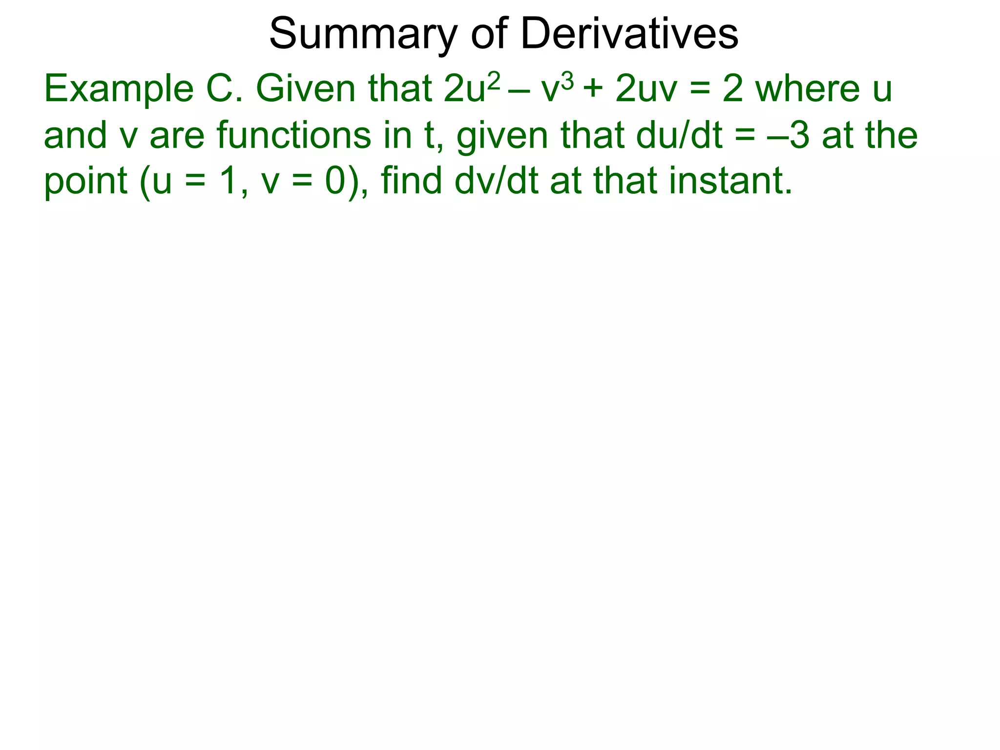
![Summary of Derivatives
Example C. Given that 2u2 – v3 + 2uv = 2 where u
and v are functions in t, given that du/dt = –3 at the
point (u = 1, v = 0), find dv/dt at that instant.
Taking the derivative with respect to t using the
prime–notation,
[2u2 – v3 + 2uv = 2]'](https://image.slidesharecdn.com/4-4reviewonderivatives-120430211412-phpapp02/75/4-4-review-on-derivatives-48-2048.jpg)
![Summary of Derivatives
Example C. Given that 2u2 – v3 + 2uv = 2 where u
and v are functions in t, given that du/dt = –3 at the
point (u = 1, v = 0), find dv/dt at that instant.
Taking the derivative with respect to t using the
prime–notation,
[2u2 – v3 + 2uv = 2]'
4uu' – 3v2v' + 2u'v + 2uv' = 0](https://image.slidesharecdn.com/4-4reviewonderivatives-120430211412-phpapp02/75/4-4-review-on-derivatives-49-2048.jpg)
![Summary of Derivatives
Example C. Given that 2u2 – v3 + 2uv = 2 where u
and v are functions in t, given that du/dt = –3 at the
point (u = 1, v = 0), find dv/dt at that instant.
Taking the derivative with respect to t using the
prime–notation,
[2u2 – v3 + 2uv = 2]'
4uu' – 3v2v' + 2u'v + 2uv' = 0
Substitute u' = –3 at u = 1, v = 0, we get
–12 + 2v' = 0](https://image.slidesharecdn.com/4-4reviewonderivatives-120430211412-phpapp02/75/4-4-review-on-derivatives-50-2048.jpg)
![Summary of Derivatives
Example C. Given that 2u2 – v3 + 2uv = 2 where u
and v are functions in t, given that du/dt = –3 at the
point (u = 1, v = 0), find dv/dt at that instant.
Taking the derivative with respect to t using the
prime–notation,
[2u2 – v3 + 2uv = 2]'
4uu' – 3v2v' + 2u'v + 2uv' = 0
Substitute u' = –3 at u = 1, v = 0, we get
–12 + 2v' = 0 or v' = dv/dt = 6](https://image.slidesharecdn.com/4-4reviewonderivatives-120430211412-phpapp02/75/4-4-review-on-derivatives-51-2048.jpg)
![Summary of Derivatives
Example C. Given that 2u2 – v3 + 2uv = 2 where u
and v are functions in t, given that du/dt = –3 at the
point (u = 1, v = 0), find dv/dt at that instant.
Taking the derivative with respect to t using the
prime–notation,
[2u2 – v3 + 2uv = 2]'
4uu' – 3v2v' + 2u'v + 2uv' = 0
Substitute u' = –3 at u = 1, v = 0, we get
–12 + 2v' = 0 or v' = dv/dt = 6
The Geometry of Derivatives](https://image.slidesharecdn.com/4-4reviewonderivatives-120430211412-phpapp02/75/4-4-review-on-derivatives-52-2048.jpg)
![Summary of Derivatives
Example C. Given that 2u2 – v3 + 2uv = 2 where u
and v are functions in t, given that du/dt = –3 at the
point (u = 1, v = 0), find dv/dt at that instant.
Taking the derivative with respect to t using the
prime–notation,
[2u2 – v3 + 2uv = 2]'
4uu' – 3v2v' + 2u'v + 2uv' = 0
Substitute u' = –3 at u = 1, v = 0, we get
–12 + 2v' = 0 or v' = dv/dt = 6
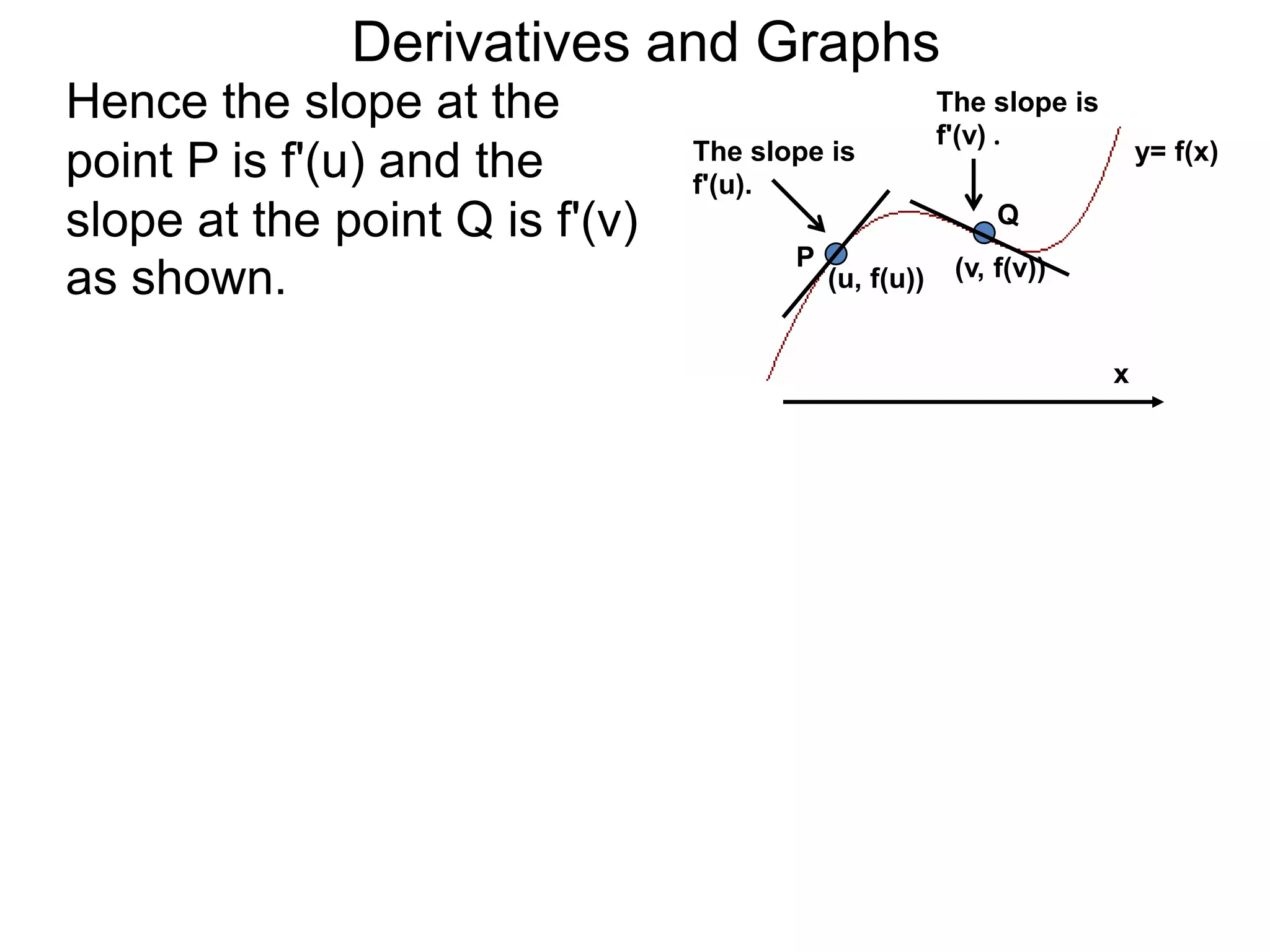
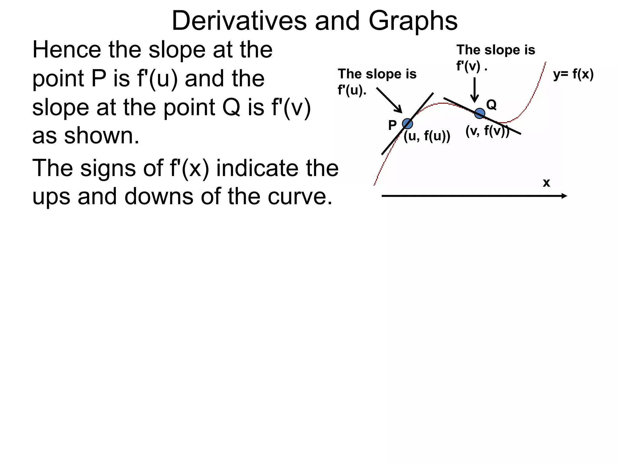
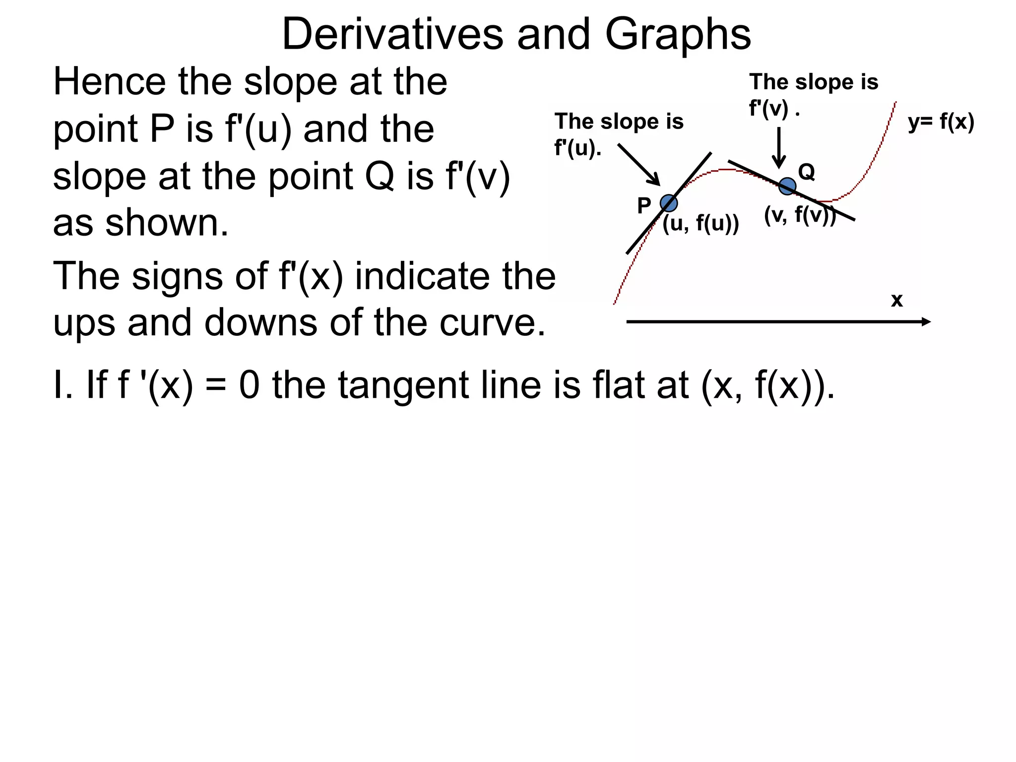
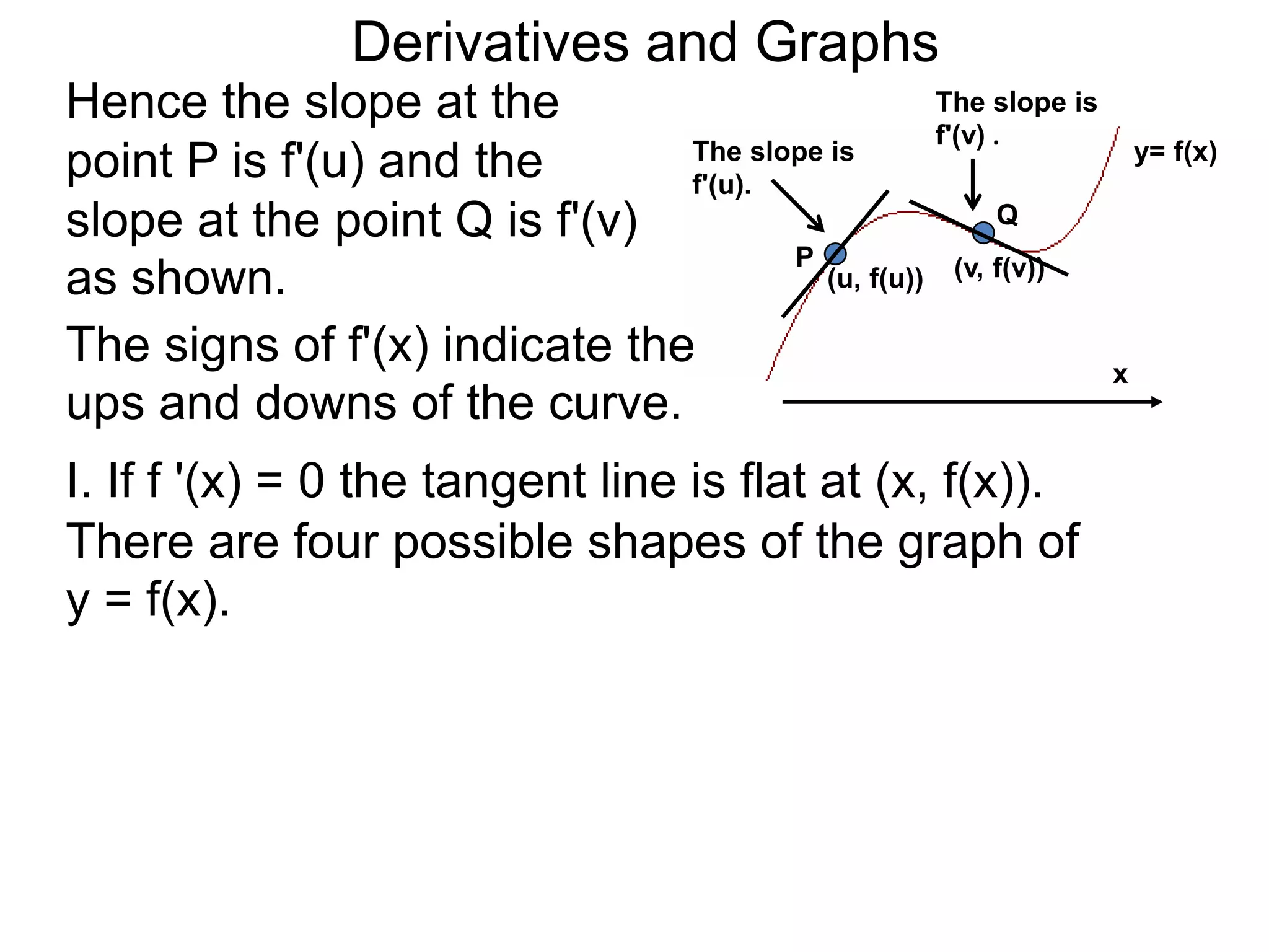
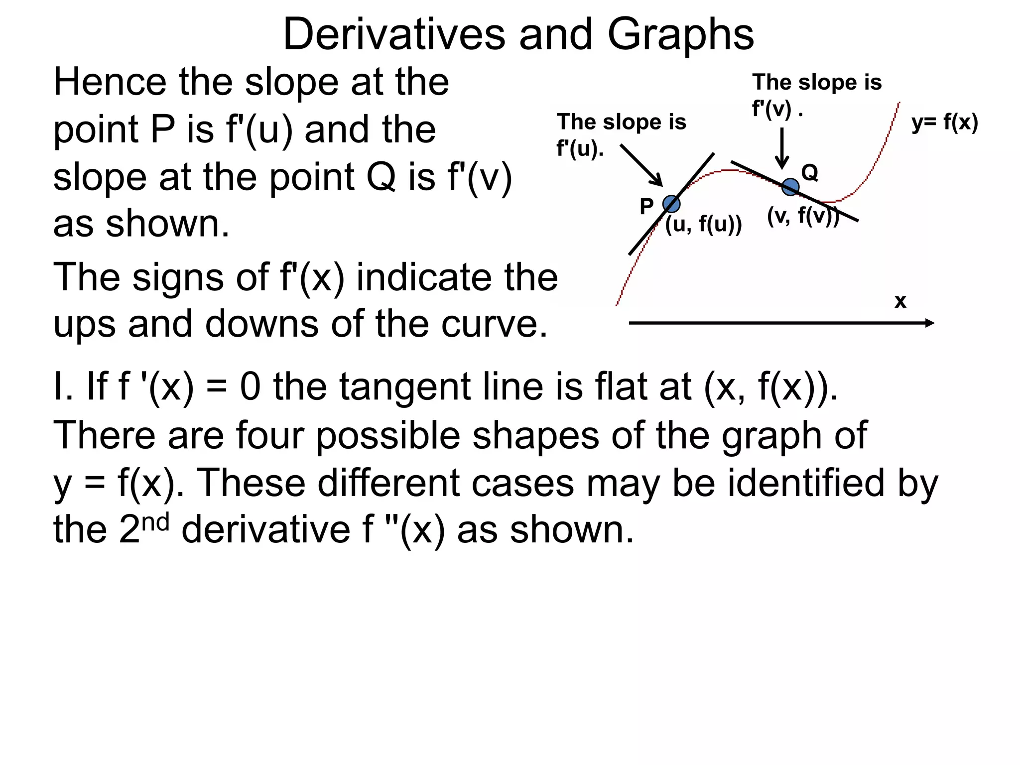
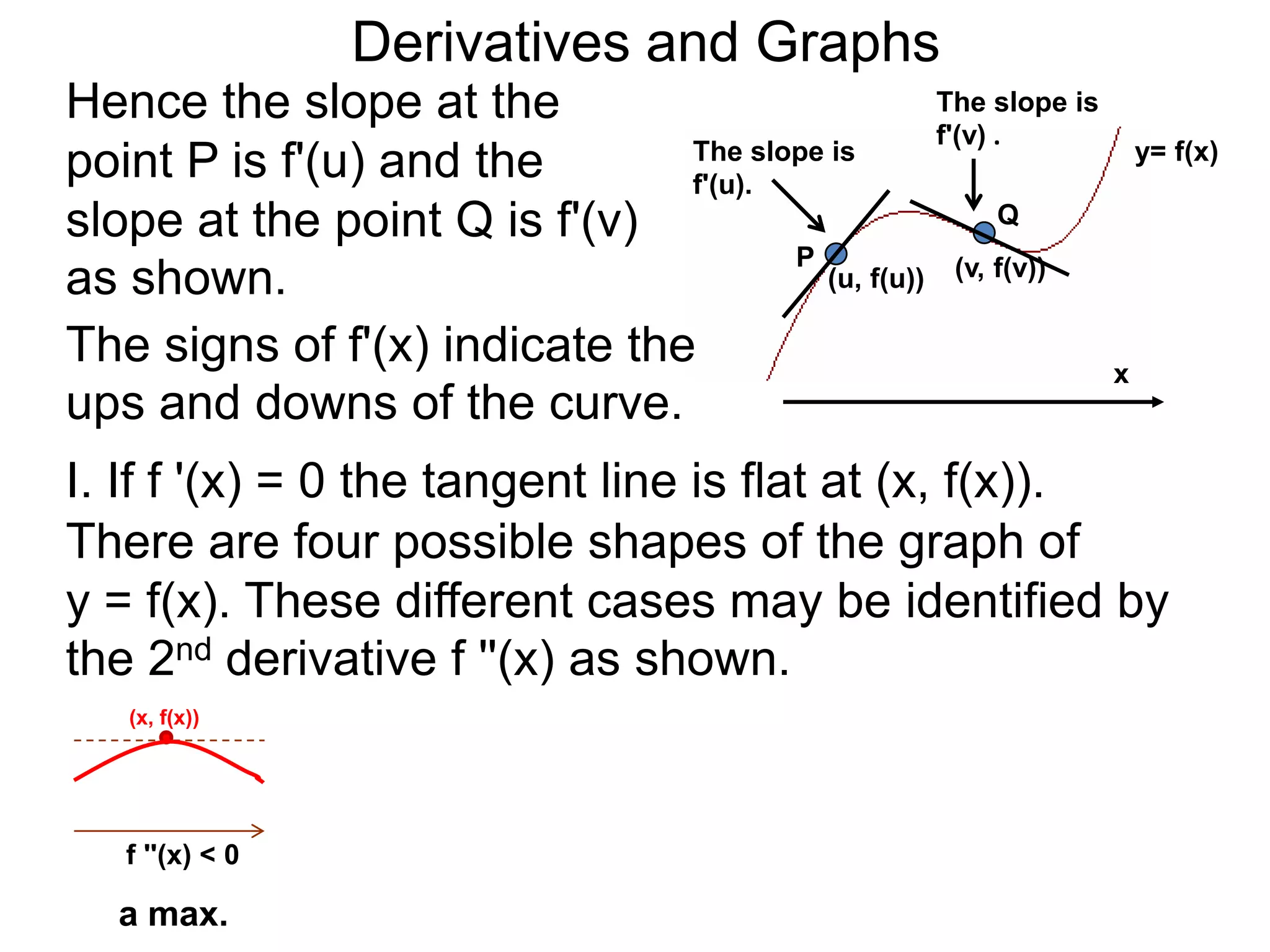
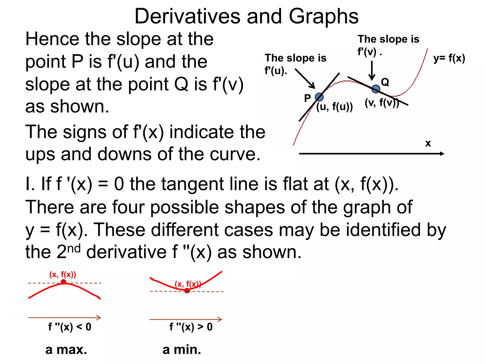
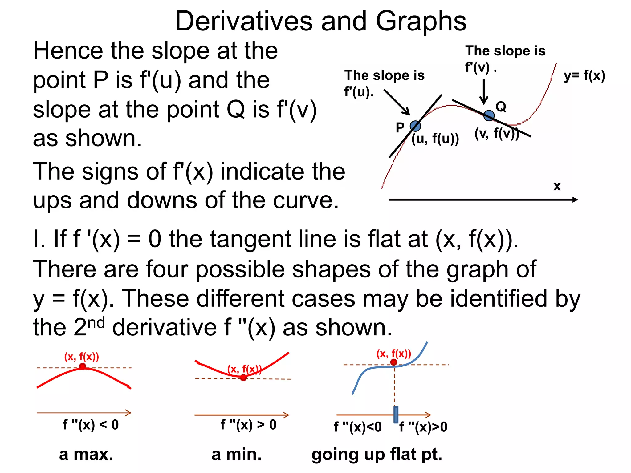
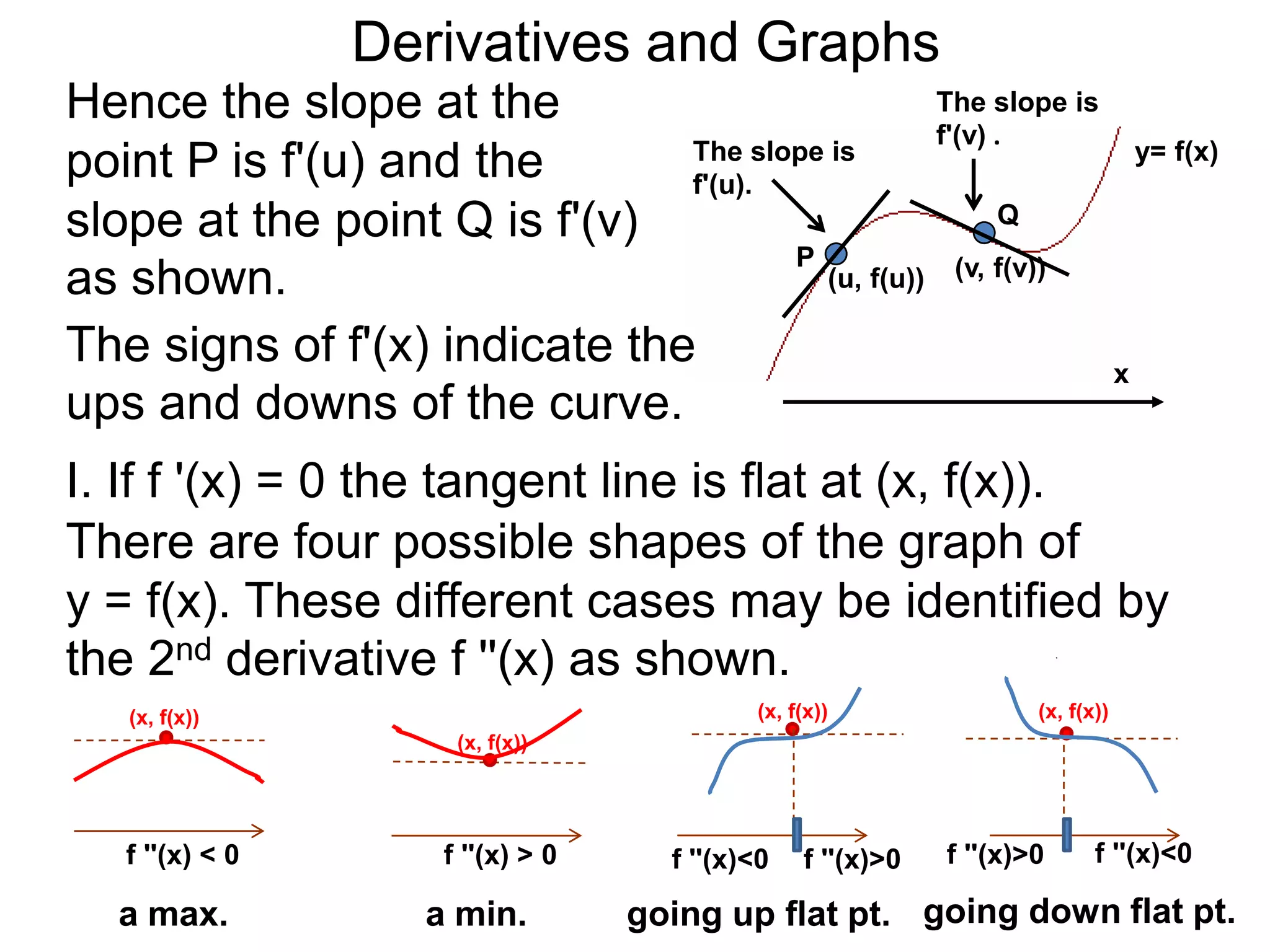
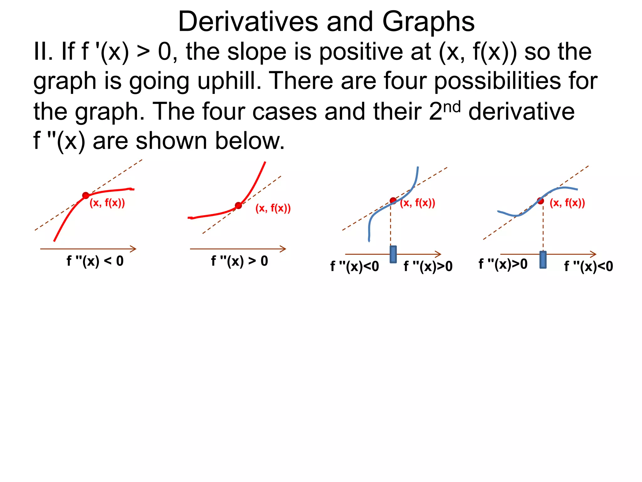
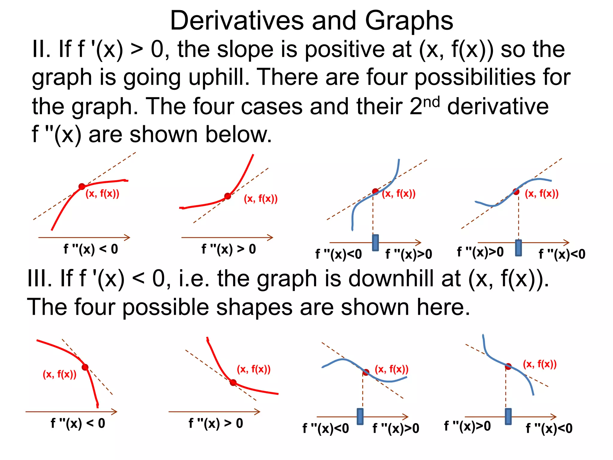
The Geometry of Derivatives
At a generic point x, the derivative f'(x) of the
function f(x) gives the “slope” at the point (x, f(x))
on the graph of y = f(x).](https://image.slidesharecdn.com/4-4reviewonderivatives-120430211412-phpapp02/75/4-4-review-on-derivatives-53-2048.jpg)
![Summary of Derivatives
Example C. Given that 2u2 – v3 + 2uv = 2 where u
and v are functions in t, given that du/dt = –3 at the
point (u = 1, v = 0), find dv/dt at that instant.
Taking the derivative with respect to t using the
prime–notation,
[2u2 – v3 + 2uv = 2]'
4uu' – 3v2v' + 2u'v + 2uv' = 0
Substitute u' = –3 at u = 1, v = 0, we get
–12 + 2v' = 0 or v' = dv/dt = 6
The Geometry of Derivatives
At a generic point x, the derivative f'(x) of the
function f(x) gives the “slope” at the point (x, f(x))
on the graph of y = f(x). The existence of this slope
means the graph is smooth at that point.](https://image.slidesharecdn.com/4-4reviewonderivatives-120430211412-phpapp02/75/4-4-review-on-derivatives-54-2048.jpg)
![Summary of Derivatives
Example C. Given that 2u2 – v3 + 2uv = 2 where u
and v are functions in t, given that du/dt = –3 at the
point (u = 1, v = 0), find dv/dt at that instant.
Taking the derivative with respect to t using the
prime–notation,
[2u2 – v3 + 2uv = 2]'
4uu' – 3v2v' + 2u'v + 2uv' = 0
Substitute u' = –3 at u = 1, v = 0, we get
–12 + 2v' = 0 or v' = dv/dt = 6
The Geometry of Derivatives
At a generic point x, the derivative f'(x) of the
function f(x) gives the “slope” at the point (x, f(x))
on the graph of y = f(x). The existence of this slope
means the graph is smooth at that point.](https://image.slidesharecdn.com/4-4reviewonderivatives-120430211412-phpapp02/75/4-4-review-on-derivatives-55-2048.jpg)
![Summary of Derivatives
Example D. Given that 2u2 – v3 = 2v + 3 draw the
graph of v = v(u) near the point (u, v) = (0, –1).
Take the derivative with respect to u to find dv/du,
[2u2 – v3 = 2v + 3] '](https://image.slidesharecdn.com/4-4reviewonderivatives-120430211412-phpapp02/75/4-4-review-on-derivatives-68-2048.jpg)
![Summary of Derivatives
Example D. Given that 2u2 – v3 = 2v + 3 draw the
graph of v = v(u) near the point (u, v) = (0, –1).
Take the derivative with respect to u to find dv/du,
[2u2 – v3 = 2v + 3] ' 4u – 3v2v' = 2v'](https://image.slidesharecdn.com/4-4reviewonderivatives-120430211412-phpapp02/75/4-4-review-on-derivatives-69-2048.jpg)
![Summary of Derivatives
Example D. Given that 2u2 – v3 = 2v + 3 draw the
graph of v = v(u) near the point (u, v) = (0, –1).
Take the derivative with respect to u to find dv/du,
[2u2 – v3 = 2v + 3] ' 4u – 3v2v' = 2v'
So v' = 2 4u 2
+ 3v](https://image.slidesharecdn.com/4-4reviewonderivatives-120430211412-phpapp02/75/4-4-review-on-derivatives-70-2048.jpg)
![Summary of Derivatives
Example D. Given that 2u2 – v3 = 2v + 3 draw the
graph of v = v(u) near the point (u, v) = (0, –1).
Take the derivative with respect to u to find dv/du,
[2u2 – v3 = 2v + 3] ' 4u – 3v2v' = 2v'
So v' = 2 4u 2
+ 3v
At u = 0, v = –1, we get v' = 0.](https://image.slidesharecdn.com/4-4reviewonderivatives-120430211412-phpapp02/75/4-4-review-on-derivatives-71-2048.jpg)
![Summary of Derivatives
Example D. Given that 2u2 – v3 = 2v + 3 draw the
graph of v = v(u) near the point (u, v) = (0, –1).
Take the derivative with respect to u to find dv/du,
[2u2 – v3 = 2v + 3] ' 4u – 3v2v' = 2v'
So v' = 2 4u 2
+ 3v
At u = 0, v = –1, we get v' = 0.
Take the derivative of v' with respect to u again, we get](https://image.slidesharecdn.com/4-4reviewonderivatives-120430211412-phpapp02/75/4-4-review-on-derivatives-72-2048.jpg)
![Summary of Derivatives
Example D. Given that 2u2 – v3 = 2v + 3 draw the
graph of v = v(u) near the point (u, v) = (0, –1).
Take the derivative with respect to u to find dv/du,
[2u2 – v3 = 2v + 3] ' 4u – 3v2v' = 2v'
So v' = 2 4u 2
+ 3v
At u = 0, v = –1, we get v' = 0.
Take the derivative of v' with respect to u again, we get
So v'' =
(2 + 3v2)2](https://image.slidesharecdn.com/4-4reviewonderivatives-120430211412-phpapp02/75/4-4-review-on-derivatives-73-2048.jpg)
![Summary of Derivatives
Example D. Given that 2u2 – v3 = 2v + 3 draw the
graph of v = v(u) near the point (u, v) = (0, –1).
Take the derivative with respect to u to find dv/du,
[2u2 – v3 = 2v + 3] ' 4u – 3v2v' = 2v'
So v' = 2 4u 2
+ 3v
At u = 0, v = –1, we get v' = 0.
Take the derivative of v' with respect to u again, we get
So v'' = (2 + 3v2)(4) – 4u(6vv')
(2 + 3v2)2](https://image.slidesharecdn.com/4-4reviewonderivatives-120430211412-phpapp02/75/4-4-review-on-derivatives-74-2048.jpg)
![Summary of Derivatives
Example D. Given that 2u2 – v3 = 2v + 3 draw the
graph of v = v(u) near the point (u, v) = (0, –1).
Take the derivative with respect to u to find dv/du,
[2u2 – v3 = 2v + 3] ' 4u – 3v2v' = 2v'
So v' = 2 4u 2
+ 3v
At u = 0, v = –1, we get v' = 0.
Take the derivative of v' with respect to u again, we get
So v'' = (2 + 3v2)(4) – 4u(6vv')
(2 + 3v2)2
At u = 0, v = –1, and v' = 0 we get
v'' > 0.](https://image.slidesharecdn.com/4-4reviewonderivatives-120430211412-phpapp02/75/4-4-review-on-derivatives-75-2048.jpg)
![Summary of Derivatives
Example D. Given that 2u2 – v3 = 2v + 3 draw the
graph of v = v(u) near the point (u, v) = (0, –1).
Take the derivative with respect to u to find dv/du,
[2u2 – v3 = 2v + 3] ' 4u – 3v2v' = 2v'
So v' = 2 4u 2
+ 3v
At u = 0, v = –1, we get v' = 0.
Take the derivative of v' with respect to u again, we get
So v'' = (2 + 3v2)(4) – 4u(6vv')
(2 + 3v2)2
At u = 0, v = –1, and v' = 0 we get
v'' > 0. From these, we conclude that
(0, –1) must be a minimum.](https://image.slidesharecdn.com/4-4reviewonderivatives-120430211412-phpapp02/75/4-4-review-on-derivatives-76-2048.jpg)
![Summary of Derivatives
Example D. Given that 2u2 – v3 = 2v + 3 draw the
graph of v = v(u) near the point (u, v) = (0, –1).
Take the derivative with respect to u to find dv/du,
[2u2 – v3 = 2v + 3] ' 4u – 3v2v' = 2v'
So v' = 2 4u 2
+ 3v
At u = 0, v = –1, we get v' = 0.
Take the derivative of v' with respect to u again, we get
So v'' = (2 + 3v2)(4) – 4u(6vv') v
(2 + 3v2)2
At u = 0, v = –1, and v' = 0 we get u
v'' > 0. From these, we conclude that (0,–1)
(0, –1) must be a minimum. v'(0) = 0
v''(0) > 0](https://image.slidesharecdn.com/4-4reviewonderivatives-120430211412-phpapp02/75/4-4-review-on-derivatives-77-2048.jpg)