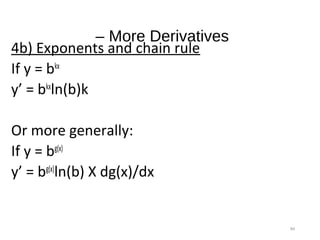
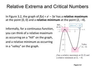
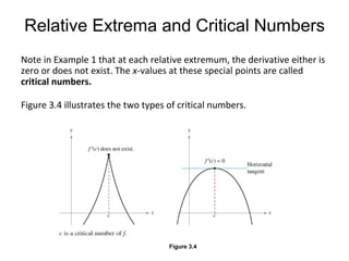
This document discusses derivatives and their rules and applications. It begins by defining the derivative and tangent line, then presents the power rule, constant multiple rule, sum and difference rules, and product, quotient, and chain rules for differentiation. It also covers higher order derivatives, derivatives of trigonometric functions, and applications of derivatives like velocity, acceleration, marginal cost, and rates of change.


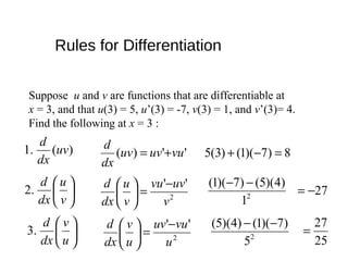


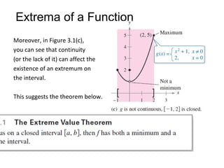
![A function need not have a minimum or a maximum on an interval. For
instance, in Figure 3.1(a) and (b), you can see that the function f(x) = x2
+ 1
has both a minimum and a maximum on the closed interval [–1, 2], but
does not have a maximum on the open interval (–1, 2).
Figure 3.1(a) Figure 3.1(b)
Extrema of a Function](https://image.slidesharecdn.com/differential-calculus-181203055858/85/Differential-calculus-95-320.jpg)


![Example 1(a) – Solution
At the point (3, 2), the value of the derivative is f'(3) = 0
[see Figure 3.3(a)].
The derivative of is
Figure 3.3(a)](https://image.slidesharecdn.com/differential-calculus-181203055858/85/Differential-calculus-102-320.jpg)
![Example 1(b) – Solution
At x = 0, the derivative of f(x) = |x| does not exist because the following
one-sided limits differ [see Figure 3.3(b)].
cont’d
Figure 3.3(b)](https://image.slidesharecdn.com/differential-calculus-181203055858/85/Differential-calculus-103-320.jpg)
![Example 1(c) – Solution
The derivative of f(x) = sin x is f'(x) = cos x.
At the point (π/2, 1), the value of the
derivative is f'(π/2) = cos(π/2) = 0.
At the point (3π/2, –1), the value of the
derivative is f'(3π/2) = cos(3π/2) = 0
[see Figure 3.3(c)].
cont’d
Figure 3.3(c)](https://image.slidesharecdn.com/differential-calculus-181203055858/85/Differential-calculus-104-320.jpg)


![Example 2 – Finding Extrema on a Closed Interval
Find the extrema of f(x) = 3x4
– 4x3
on the interval [–1, 2].
Solution:
Begin by differentiating the function.
f(x) = 3x4
– 4x3
Write original function.
f'(x) = 12x3
– 12x2
Differentiate.](https://image.slidesharecdn.com/differential-calculus-181203055858/85/Differential-calculus-108-320.jpg)

![By evaluating f at these two critical numbers and at the
endpoints of [–1, 2], you can determine that the
maximum is f(2) = 16 and the minimum is f(1) = –1, as
shown in the table.
Example 2 – Solution cont’d](https://image.slidesharecdn.com/differential-calculus-181203055858/85/Differential-calculus-110-320.jpg)


![• Determine the absolute extrema for the following function and
interval[-4,2].
•](https://image.slidesharecdn.com/differential-calculus-181203055858/85/Differential-calculus-113-320.jpg)


![Library Work # 2
•1. Sketch the graph of f. Find the absolute
and local maximum and minimum values of f.
Use the interval [-1,4]
•2. f(x)= X4
+ 4x3
-2x2
-12x](https://image.slidesharecdn.com/differential-calculus-181203055858/85/Differential-calculus-125-320.jpg)