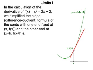
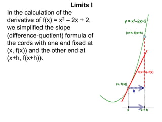
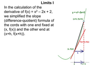
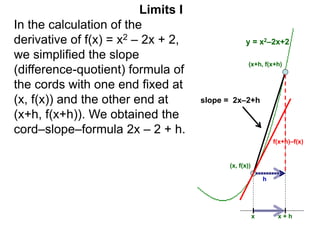
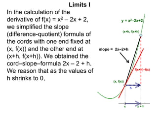
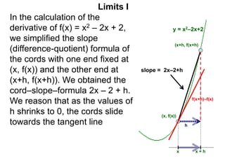
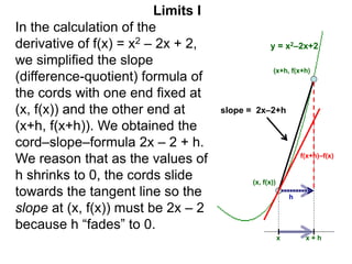
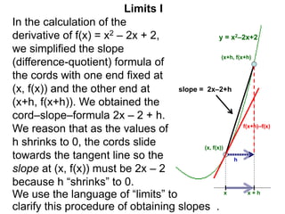
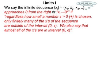
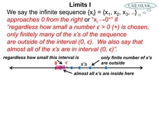
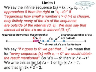
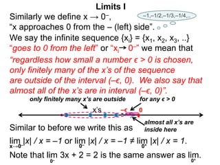
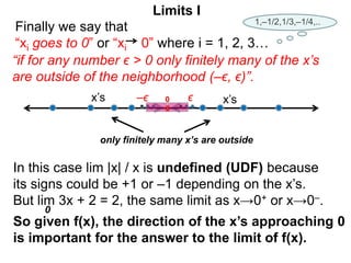
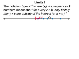
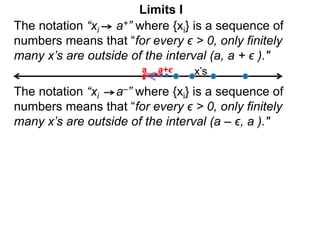
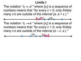
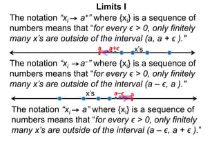
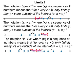
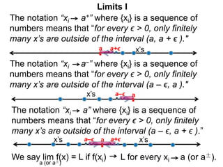
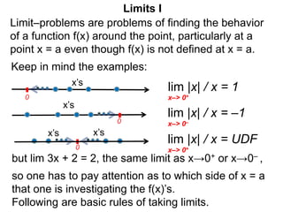
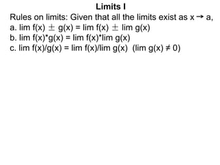
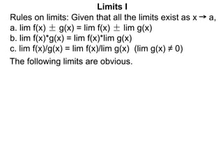
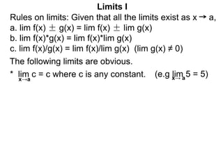
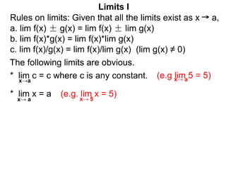
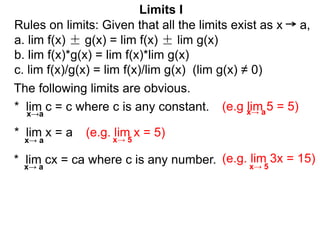
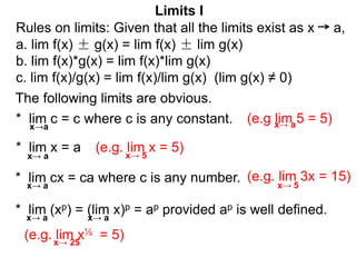
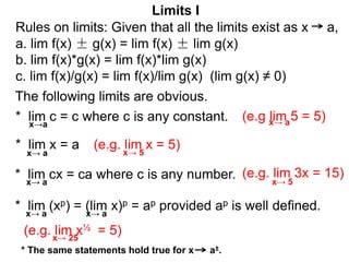
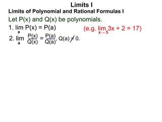
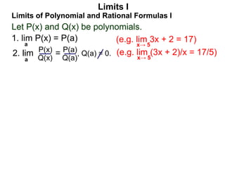
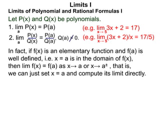
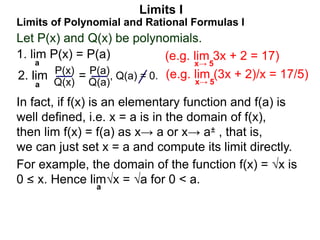
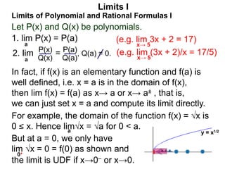
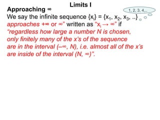
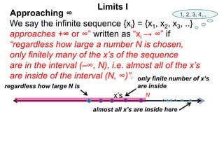
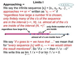
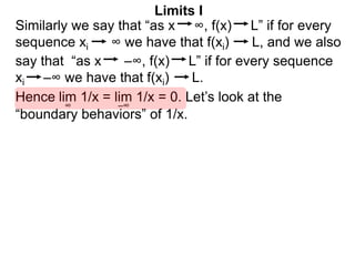
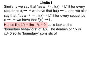
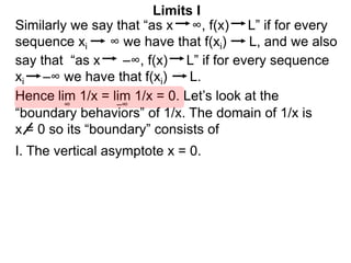
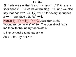
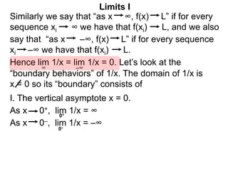
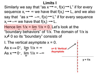
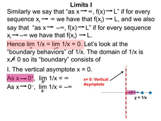
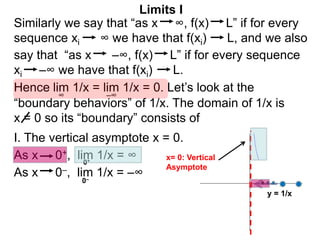
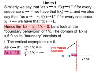
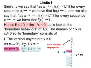
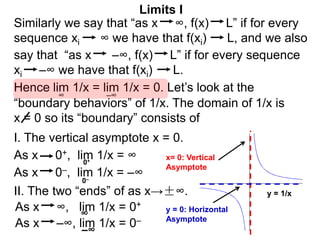
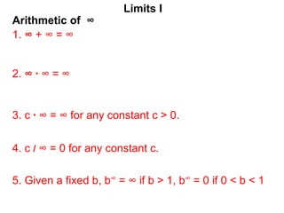
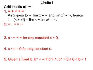
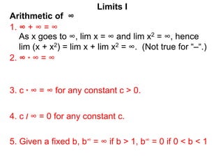
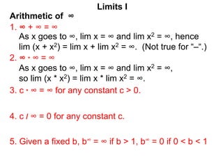
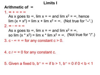
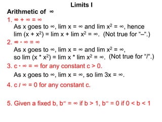
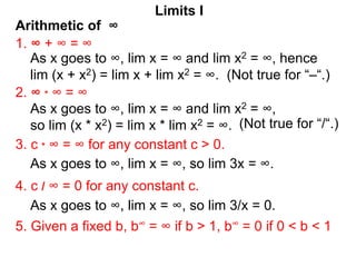
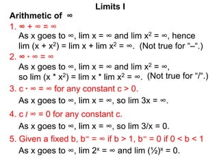
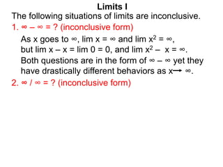
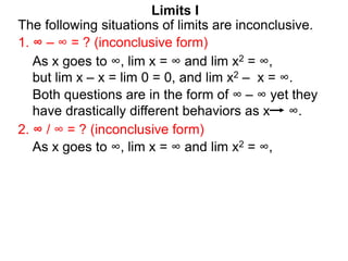
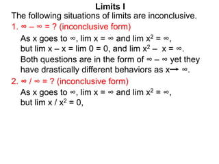
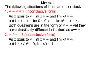
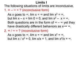
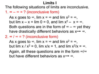
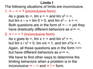
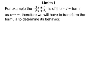
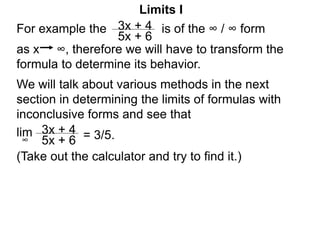
The document discusses limits and how they are used to calculate the derivative of a function. It defines what it means for a sequence to approach a limit from the right or left side. Graphs and examples are provided to illustrate these concepts. The key rules for calculating limits are outlined, such as using algebra to split limits into their constituent parts. Common types of obvious limits are also stated, such as limits of constants or products involving constants.

1. Limits I

2. Limits I
In the calculation of the
derivative of f(x) = x2 – 2x + 2,
we simplified the slope
(difference-quotient) formula of
the cords with one end fixed at
(x, f(x)) and the other end at
(x+h, f(x+h)).
(x, f(x))
x
y = x2–2x+2

3. Limits I
In the calculation of the
derivative of f(x) = x2 – 2x + 2,
we simplified the slope
(difference-quotient) formula of
the cords with one end fixed at
(x, f(x)) and the other end at
(x+h, f(x+h)).
(x+h, f(x+h)
(x, f(x))
x x + h
f(x+h)–f(x)
h
y = x2–2x+2

4. Limits I
In the calculation of the
derivative of f(x) = x2 – 2x + 2,
we simplified the slope
(difference-quotient) formula of
the cords with one end fixed at
(x, f(x)) and the other end at
(x+h, f(x+h)).
(x+h, f(x+h)
(x, f(x))
x x + h
f(x+h)–f(x)
h
y = x2–2x+2

5. Limits I
In the calculation of the
derivative of f(x) = x2 – 2x + 2,
we simplified the slope
(difference-quotient) formula of
the cords with one end fixed at
(x, f(x)) and the other end at
(x+h, f(x+h)). We obtained the
cord–slope–formula 2x – 2 + h.
(x+h, f(x+h)
(x, f(x))
x x + h
f(x+h)–f(x)
h
y = x2–2x+2
slope = 2x–2+h

6. Limits I
In the calculation of the
derivative of f(x) = x2 – 2x + 2,
we simplified the slope
(difference-quotient) formula of
the cords with one end fixed at
(x, f(x)) and the other end at
(x+h, f(x+h)). We obtained the
cord–slope–formula 2x – 2 + h.
We reason that as the values of
h shrinks to 0,
(x+h, f(x+h)
(x, f(x))
x x + h
f(x+h)–f(x)
h
y = x2–2x+2
slope = 2x–2+h

7. Limits I
In the calculation of the
derivative of f(x) = x2 – 2x + 2,
we simplified the slope
(difference-quotient) formula of
the cords with one end fixed at
(x, f(x)) and the other end at
(x+h, f(x+h)). We obtained the
cord–slope–formula 2x – 2 + h.
We reason that as the values of
h shrinks to 0, the cords slide
towards the tangent line
(x+h, f(x+h)
(x, f(x))
x x + h
f(x+h)–f(x)
h
y = x2–2x+2
slope = 2x–2+h

8. Limits I
In the calculation of the
derivative of f(x) = x2 – 2x + 2,
we simplified the slope
(difference-quotient) formula of
the cords with one end fixed at
(x, f(x)) and the other end at
(x+h, f(x+h)). We obtained the
cord–slope–formula 2x – 2 + h.
We reason that as the values of
h shrinks to 0, the cords slide
towards the tangent line so the
slope at (x, f(x)) must be 2x – 2
because h “fades” to 0.
(x+h, f(x+h)
(x, f(x))
x x + h
f(x+h)–f(x)
h
y = x2–2x+2
slope = 2x–2+h

9. Limits I
In the calculation of the
derivative of f(x) = x2 – 2x + 2,
we simplified the slope
(difference-quotient) formula of
the cords with one end fixed at
(x, f(x)) and the other end at
(x+h, f(x+h)). We obtained the
cord–slope–formula 2x – 2 + h.
We reason that as the values of
h shrinks to 0, the cords slide
towards the tangent line so the
slope at (x, f(x)) must be 2x – 2
because h “shrinks” to 0.
(x+h, f(x+h)
(x, f(x))
x x + h
f(x+h)–f(x)
h
y = x2–2x+2
slope = 2x–2+h
clarify this procedure of obtaining slopes .
We use the language of “limits” to

10. We say the infinite sequence {xi} = {x1, x2, x3, ..}
approaches 0 from the right or “xi →0+” if
“regardless how small a number ϵ > 0 (+) is chosen,
only finitely many of the x’s of the sequence
are outside of the interval (0, ϵ). We also say that
almost all of the x’s are in interval (0, ϵ)”.
Limits I 1,1/2,1/3,1/4,..

11. We say the infinite sequence {xi} = {x1, x2, x3, ..}
approaches 0 from the right or “xi →0+” if
“regardless how small a number ϵ > 0 (+) is chosen,
only finitely many of the x’s of the sequence
are outside of the interval (0, ϵ). We also say that
almost all of the x’s are in interval (0, ϵ)”.
0 x’s
ϵ
only finite number of x’s
are outside
regardless how small this interval is
Limits I
almost all x’s are inside here
1,1/2,1/3,1/4,..

12. We say the infinite sequence {xi} = {x1, x2, x3, ..}
approaches 0 from the right or “xi →0+” if
“regardless how small a number ϵ > 0 (+) is chosen,
only finitely many of the x’s of the sequence
are outside of the interval (0, ϵ). We also say that
almost all of the x’s are in interval (0, ϵ)”.
We say “if x goes to 0+ we get that …” we mean that
for “every sequence {xi} with xi → 0+ we would obtain
the result mentioned”. So “if x → 0+ then |x| / x →1”
We write this as lim |x| / x = 1 or lim |x| / x = 1,
0+
0 x’s
ϵ
only finite number of x’s
are outside
regardless how small this interval is
Limits I
x→0+
almost all x’s are inside here
and that lim 3x + 2 = 2.
0+
1,1/2,1/3,1/4,..

13. We say the infinite sequence {xi} = {x1, x2, x3, ..}
“goes to 0 from the left” or “xi 0–” we mean that
Similarly we define x → 0–,
“x approaches 0 from the – (left) side”.
“regardless how small a number ϵ > 0 is chosen,
only finitely many of the x’s of the sequence
are outside of the interval (–ϵ, 0). We also say that
almost all of the x’s are in interval (–ϵ, 0)”.
only finitely many x’s are outside for any ϵ > 0
Limits I
0
x’s –ϵ
Similar to before we write this as
lim |x| / x = –1 or lim |x| / x = –1 ≠ lim |x| / x = 1.
0–
x→0–
Note that lim 3x + 2 = 2 is the same answer as lim.
0– 0+
0+
almost all x’s are
inside here
–1,–1/2,–1/3,–1/4,..

14. Finally we say that
“xi goes to 0” or “xi 0” where i = 1, 2, 3…
In this case lim |x| / x is undefined (UDF) because
its signs could be +1 or –1 depending on the x’s.
But lim 3x + 2 = 2, the same limit as x→0+ or x→0–.
So given f(x), the direction of the x’s approaching 0
is important for the answer to the limit of f(x).
“if for any number ϵ > 0 only finitely many of the x’s
are outside of the neighborhood (–ϵ, ϵ)”.
0
x’s –ϵ
only finitely many x’s are outside
x’s
ϵ
0
Limits I
1,–1/2,1/3,–1/4,..

15. The notation “xi a+” where {xi} is a sequence of
numbers means that “for every ϵ > 0, only finitely
many x’s are outside of the interval (a, a + ϵ )."
Limits I

16. The notation “xi a+” where {xi} is a sequence of
numbers means that “for every ϵ > 0, only finitely
many x’s are outside of the interval (a, a + ϵ )."
a x’s
a+ϵ
Limits I

17. The notation “xi a+” where {xi} is a sequence of
numbers means that “for every ϵ > 0, only finitely
many x’s are outside of the interval (a, a + ϵ )."
a x’s
a+ϵ
Limits I
The notation “xi a–” where {xi} is a sequence of
numbers means that “for every ϵ > 0, only finitely
many x’s are outside of the interval (a – ϵ, a )."

18. The notation “xi a+” where {xi} is a sequence of
numbers means that “for every ϵ > 0, only finitely
many x’s are outside of the interval (a, a + ϵ )."
a x’s
a+ϵ
a
x’s a–ϵ
Limits I
The notation “xi a–” where {xi} is a sequence of
numbers means that “for every ϵ > 0, only finitely
many x’s are outside of the interval (a – ϵ, a )."

19. The notation “xi a+” where {xi} is a sequence of
numbers means that “for every ϵ > 0, only finitely
many x’s are outside of the interval (a, a + ϵ )."
a x’s
a+ϵ
a
x’s a–ϵ
Limits I
The notation “xi a–” where {xi} is a sequence of
numbers means that “for every ϵ > 0, only finitely
many x’s are outside of the interval (a – ϵ, a )."
The notation “xi a” where {xi} is a sequence of
numbers means that “for every ϵ > 0, only finitely
many x’s are outside of the interval (a – ϵ, a + ϵ ).”

20. The notation “xi a+” where {xi} is a sequence of
numbers means that “for every ϵ > 0, only finitely
many x’s are outside of the interval (a, a + ϵ )."
a x’s
a+ϵ
a
x’s a–ϵ
Limits I
The notation “xi a–” where {xi} is a sequence of
numbers means that “for every ϵ > 0, only finitely
many x’s are outside of the interval (a – ϵ, a )."
The notation “xi a” where {xi} is a sequence of
numbers means that “for every ϵ > 0, only finitely
many x’s are outside of the interval (a – ϵ, a + ϵ ).”
a
x’s a–ϵ a+ϵ x’s

21. The notation “xi a+” where {xi} is a sequence of
numbers means that “for every ϵ > 0, only finitely
many x’s are outside of the interval (a, a + ϵ )."
a x’s
a+ϵ
a
x’s a–ϵ
Limits I
The notation “xi a–” where {xi} is a sequence of
numbers means that “for every ϵ > 0, only finitely
many x’s are outside of the interval (a – ϵ, a )."
The notation “xi a” where {xi} is a sequence of
numbers means that “for every ϵ > 0, only finitely
many x’s are outside of the interval (a – ϵ, a + ϵ ).”
a
x’s a–ϵ a+ϵ x’s
We say lim f(x) = L if f(xi) L for every xi a (or a±).
a (or a±)

22. Keep in mind the examples:
x’s
Limits I
lim |x| / x = 1
0 x–> 0+
lim |x| / x = –1
x–> 0–
x’s
0
lim |x| / x = UDF
x–> 0+
0
x’s
x’s
but lim 3x + 2 = 2, the same limit as x→0+ or x→0– ,
Limit–problems are problems of finding the behavior
of a function f(x) around the point, particularly at a
point x = a even though f(x) is not defined at x = a.
so one has to pay attention as to which side of x = a
that one is investigating the f(x)’s.
Following are basic rules of taking limits.

23. Limits I
Rules on limits: Given that all the limits exist as x a,
a. lim f(x) ± g(x) = lim f(x) ± lim g(x)
b. lim f(x)*g(x) = lim f(x)*lim g(x)
c. lim f(x)/g(x) = lim f(x)/lim g(x) (lim g(x) ≠ 0)

24. The following limits are obvious.
Limits I
Rules on limits: Given that all the limits exist as x a,
a. lim f(x) ± g(x) = lim f(x) ± lim g(x)
b. lim f(x)*g(x) = lim f(x)*lim g(x)
c. lim f(x)/g(x) = lim f(x)/lim g(x) (lim g(x) ≠ 0)

25. The following limits are obvious.
* lim c = c where c is any constant.
x→a
(e.g lim 5 = 5)
Limits I
x→ a
Rules on limits: Given that all the limits exist as x a,
a. lim f(x) ± g(x) = lim f(x) ± lim g(x)
b. lim f(x)*g(x) = lim f(x)*lim g(x)
c. lim f(x)/g(x) = lim f(x)/lim g(x) (lim g(x) ≠ 0)

26. The following limits are obvious.
* lim c = c where c is any constant.
x→a
* lim x = a
(e.g lim 5 = 5)
(e.g. lim x = 5)
Limits I
x→ a
x→ a x→ 5
Rules on limits: Given that all the limits exist as x a,
a. lim f(x) ± g(x) = lim f(x) ± lim g(x)
b. lim f(x)*g(x) = lim f(x)*lim g(x)
c. lim f(x)/g(x) = lim f(x)/lim g(x) (lim g(x) ≠ 0)

27. The following limits are obvious.
* lim c = c where c is any constant.
x→a
* lim x = a
* lim cx = ca where c is any number.
(e.g lim 5 = 5)
(e.g. lim x = 5)
(e.g. lim 3x = 15)
Limits I
x→ a
x→ a
x→ a
x→ 5
x→ 5
Rules on limits: Given that all the limits exist as x a,
a. lim f(x) ± g(x) = lim f(x) ± lim g(x)
b. lim f(x)*g(x) = lim f(x)*lim g(x)
c. lim f(x)/g(x) = lim f(x)/lim g(x) (lim g(x) ≠ 0)

28. * lim (xp) = (lim x)p = ap provided ap is well defined.
The following limits are obvious.
* lim c = c where c is any constant.
x→a
* lim x = a
* lim cx = ca where c is any number.
(e.g lim 5 = 5)
(e.g. lim x = 5)
(e.g. lim x½ = 5)
(e.g. lim 3x = 15)
Limits I
x→ a
x→ a
x→ a
x→ a
x→ 5
x→ 5
x→ a
x→ 25
Rules on limits: Given that all the limits exist as x a,
a. lim f(x) ± g(x) = lim f(x) ± lim g(x)
b. lim f(x)*g(x) = lim f(x)*lim g(x)
c. lim f(x)/g(x) = lim f(x)/lim g(x) (lim g(x) ≠ 0)

29. * lim (xp) = (lim x)p = ap provided ap is well defined.
The following limits are obvious.
* lim c = c where c is any constant.
x→a
* lim x = a
* lim cx = ca where c is any number.
(e.g lim 5 = 5)
(e.g. lim x = 5)
(e.g. lim x½ = 5)
(e.g. lim 3x = 15)
* The same statements hold true for x a±.
Limits I
x→ a
x→ a
x→ a
x→ a
x→ 5
x→ 5
x→ a
x→ 25
Rules on limits: Given that all the limits exist as x a,
a. lim f(x) ± g(x) = lim f(x) ± lim g(x)
b. lim f(x)*g(x) = lim f(x)*lim g(x)
c. lim f(x)/g(x) = lim f(x)/lim g(x) (lim g(x) ≠ 0)

30. Let P(x) and Q(x) be polynomials.
1. lim P(x) = P(a)
a
Limits of Polynomial and Rational Formulas I
2. lim =
P(x)
Q(x)
P(a)
Q(a)
, Q(a) = 0.
Limits I
a
(e.g. lim 3x + 2 = 17)
x→ 5

31. Let P(x) and Q(x) be polynomials.
1. lim P(x) = P(a)
a
Limits of Polynomial and Rational Formulas I
2. lim =
P(x)
Q(x)
P(a)
Q(a)
, Q(a) = 0.
Limits I
a
(e.g. lim 3x + 2 = 17)
x→ 5
(e.g. lim (3x + 2)/x = 17/5)
x→ 5

32. Let P(x) and Q(x) be polynomials.
1. lim P(x) = P(a)
a
Limits of Polynomial and Rational Formulas I
2. lim =
P(x)
Q(x)
P(a)
Q(a)
, Q(a) = 0.
Limits I
a
(e.g. lim 3x + 2 = 17)
x→ 5
(e.g. lim (3x + 2)/x = 17/5)
x→ 5
In fact, if f(x) is an elementary function and f(a) is
well defined, i.e. x = a is in the domain of f(x),
then lim f(x) = f(a) as x→ a or x→ a± , that is,
we can just set x = a and compute its limit directly.

33. Let P(x) and Q(x) be polynomials.
1. lim P(x) = P(a)
a
Limits of Polynomial and Rational Formulas I
2. lim =
P(x)
Q(x)
P(a)
Q(a)
, Q(a) = 0.
In fact, if f(x) is an elementary function and f(a) is
well defined, i.e. x = a is in the domain of f(x),
then lim f(x) = f(a) as x→ a or x→ a± , that is,
we can just set x = a and compute its limit directly.
For example, the domain of the function f(x) = √x is
0 < x. Hence lim√x = √a for 0 < a.
– a
Limits I
a
(e.g. lim 3x + 2 = 17)
x→ 5
(e.g. lim (3x + 2)/x = 17/5)
x→ 5

34. Let P(x) and Q(x) be polynomials.
1. lim P(x) = P(a)
a
Limits of Polynomial and Rational Formulas I
2. lim =
P(x)
Q(x)
P(a)
Q(a)
, Q(a) = 0.
For example, the domain of the function f(x) = √x is
0 < x. Hence lim√x = √a for 0 < a.
– a
But at a = 0, we only have
lim √x = 0 = f(0) as shown and
the limit is UDF if x→0– or x→0.
y = x1/2
0+
Limits I
a
(e.g. lim 3x + 2 = 17)
x→ 5
(e.g. lim (3x + 2)/x = 17/5)
x→ 5
In fact, if f(x) is an elementary function and f(a) is
well defined, i.e. x = a is in the domain of f(x),
then lim f(x) = f(a) as x→ a or x→ a± , that is,
we can just set x = a and compute its limit directly.

35. We say the infinite sequence {xi} = {x1, x2, x3, ..}
approaches +∞ or ∞” written as “xi → ∞” if
“regardless how large a number N is chosen,
only finitely many of the x’s of the sequence
are in the interval (–∞, N), i.e. almost all of the x’s
are inside of the interval (N, ∞)”.
Limits I
1, 2, 3, 4,..
Approaching ∞

36. We say the infinite sequence {xi} = {x1, x2, x3, ..}
approaches +∞ or ∞” written as “xi → ∞” if
“regardless how large a number N is chosen,
only finitely many of the x’s of the sequence
are in the interval (–∞, N), i.e. almost all of the x’s
are inside of the interval (N, ∞)”.
x’s
only finite number of x’s
are inside
regardless how large N is
Limits I
almost all x’s are inside here
1, 2, 3, 4,..
Approaching ∞
N

37. We say the infinite sequence {xi} = {x1, x2, x3, ..}
approaches +∞ or ∞” written as “xi → ∞” if
“regardless how large a number N is chosen,
only finitely many of the x’s of the sequence
are in the interval (–∞, N), i.e. almost all of the x’s
are inside of the interval (N, ∞)”.
We say “if x goes to ∞ we have that …” we mean that
for “every sequence {xi} with xi → ∞ we would obtain
the result mentioned”. So “if x → ∞ then 1 / x →0”
We write this as lim 1 / x = 0 or lim 1 / x = 0.
∞
x’s
only finite number of x’s
are inside
regardless how large N is
Limits I
x→ ∞
almost all x’s are inside here
1, 2, 3, 4,..
Approaching ∞
N

38. Similarly we say that “as x ∞, f(x) L” if for every
sequence xi ∞ we have that f(xi) L,
Limits I

39. Similarly we say that “as x ∞, f(x) L” if for every
sequence xi ∞ we have that f(xi) L, and we also
Limits I
say that “as x –∞, f(x) L” if for every sequence
xi –∞ we have that f(xi) L.

40. Similarly we say that “as x ∞, f(x) L” if for every
sequence xi ∞ we have that f(xi) L, and we also
lim 1/x = lim 1/x = 0.
∞
Limits I
Hence
say that “as x –∞, f(x) L” if for every sequence
xi –∞ we have that f(xi) L.
–∞

41. Similarly we say that “as x ∞, f(x) L” if for every
sequence xi ∞ we have that f(xi) L, and we also
lim 1/x = lim 1/x = 0. Let’s look at the
∞
Limits I
Hence
say that “as x –∞, f(x) L” if for every sequence
xi –∞ we have that f(xi) L.
–∞
“boundary behaviors” of 1/x.

42. Similarly we say that “as x ∞, f(x) L” if for every
sequence xi ∞ we have that f(xi) L, and we also
lim 1/x = lim 1/x = 0. Let’s look at the
∞
Limits I
Hence
say that “as x –∞, f(x) L” if for every sequence
xi –∞ we have that f(xi) L.
–∞
“boundary behaviors” of 1/x. The domain of 1/x is
x = 0 so its “boundary” consists of

43. Similarly we say that “as x ∞, f(x) L” if for every
sequence xi ∞ we have that f(xi) L, and we also
lim 1/x = lim 1/x = 0. Let’s look at the
∞
Limits I
Hence
say that “as x –∞, f(x) L” if for every sequence
xi –∞ we have that f(xi) L.
–∞
“boundary behaviors” of 1/x. The domain of 1/x is
x = 0 so its “boundary” consists of
I. The vertical asymptote x = 0.

44. Similarly we say that “as x ∞, f(x) L” if for every
sequence xi ∞ we have that f(xi) L, and we also
lim 1/x = lim 1/x = 0. Let’s look at the
∞
Limits I
Hence
say that “as x –∞, f(x) L” if for every sequence
xi –∞ we have that f(xi) L.
–∞
0+
As x 0+, lim 1/x = ∞
“boundary behaviors” of 1/x. The domain of 1/x is
x = 0 so its “boundary” consists of
I. The vertical asymptote x = 0.

45. Similarly we say that “as x ∞, f(x) L” if for every
sequence xi ∞ we have that f(xi) L, and we also
lim 1/x = lim 1/x = 0. Let’s look at the
∞
Limits I
Hence
say that “as x –∞, f(x) L” if for every sequence
xi –∞ we have that f(xi) L.
–∞
As x 0–, lim 1/x = –∞
0+
0–
As x 0+, lim 1/x = ∞
“boundary behaviors” of 1/x. The domain of 1/x is
x = 0 so its “boundary” consists of
I. The vertical asymptote x = 0.

46. Similarly we say that “as x ∞, f(x) L” if for every
sequence xi ∞ we have that f(xi) L, and we also
lim 1/x = lim 1/x = 0. Let’s look at the
∞
Limits I
Hence
say that “as x –∞, f(x) L” if for every sequence
xi –∞ we have that f(xi) L.
–∞
As x 0–, lim 1/x = –∞
0+
0–
As x 0+, lim 1/x = ∞
“boundary behaviors” of 1/x. The domain of 1/x is
x = 0 so its “boundary” consists of
I. The vertical asymptote x = 0.
y = 1/x
x= 0: Vertical
Asymptote

47. Similarly we say that “as x ∞, f(x) L” if for every
sequence xi ∞ we have that f(xi) L, and we also
lim 1/x = lim 1/x = 0. Let’s look at the
∞
Limits I
Hence
say that “as x –∞, f(x) L” if for every sequence
xi –∞ we have that f(xi) L.
–∞
As x 0–, lim 1/x = –∞
0+
0–
As x 0+, lim 1/x = ∞
“boundary behaviors” of 1/x. The domain of 1/x is
x = 0 so its “boundary” consists of
I. The vertical asymptote x = 0.
y = 1/x
x= 0: Vertical
Asymptote

48. Similarly we say that “as x ∞, f(x) L” if for every
sequence xi ∞ we have that f(xi) L, and we also
lim 1/x = lim 1/x = 0. Let’s look at the
∞
Limits I
Hence
say that “as x –∞, f(x) L” if for every sequence
xi –∞ we have that f(xi) L.
–∞
As x 0–, lim 1/x = –∞
0+
0–
As x 0+, lim 1/x = ∞
“boundary behaviors” of 1/x. The domain of 1/x is
x = 0 so its “boundary” consists of
I. The vertical asymptote x = 0.
y = 1/x
x= 0: Vertical
Asymptote

49. Similarly we say that “as x ∞, f(x) L” if for every
sequence xi ∞ we have that f(xi) L, and we also
lim 1/x = lim 1/x = 0. Let’s look at the
∞
Limits I
Hence
say that “as x –∞, f(x) L” if for every sequence
xi –∞ we have that f(xi) L.
–∞
As x 0–, lim 1/x = –∞
0+
0–
As x 0+, lim 1/x = ∞
“boundary behaviors” of 1/x. The domain of 1/x is
x = 0 so its “boundary” consists of
I. The vertical asymptote x = 0.
y = 1/x
x= 0: Vertical
Asymptote

50. Similarly we say that “as x ∞, f(x) L” if for every
sequence xi ∞ we have that f(xi) L, and we also
lim 1/x = lim 1/x = 0. Let’s look at the
∞
Limits I
Hence
say that “as x –∞, f(x) L” if for every sequence
xi –∞ we have that f(xi) L.
–∞
As x 0–, lim 1/x = –∞
0+
0–
As x 0+, lim 1/x = ∞
“boundary behaviors” of 1/x. The domain of 1/x is
x = 0 so its “boundary” consists of
I. The vertical asymptote x = 0.
y = 1/x
x= 0: Vertical
Asymptote

51. Similarly we say that “as x ∞, f(x) L” if for every
sequence xi ∞ we have that f(xi) L, and we also
lim 1/x = lim 1/x = 0. Let’s look at the
∞
Limits I
Hence
say that “as x –∞, f(x) L” if for every sequence
xi –∞ we have that f(xi) L.
–∞
As x 0–, lim 1/x = –∞
0+
0–
As x ∞, lim 1/x = 0+
∞
As x –∞, lim 1/x = 0–
–∞
As x 0+, lim 1/x = ∞
“boundary behaviors” of 1/x. The domain of 1/x is
x = 0 so its “boundary” consists of
I. The vertical asymptote x = 0.
y = 1/x
x= 0: Vertical
Asymptote
y = 0: Horizontal
Asymptote
II. The two “ends” of as x→±∞.

52. Arithmetic of ∞
Limits I

53. Arithmetic of ∞
Limits I
The symbol “∞” is not a number because it does not
represent a numerical measurement.

54. Arithmetic of ∞
Limits I
The symbol “∞” is not a number because it does not
represent a numerical measurement. It represents the
behavior of a list of endless numbers, specifically
eventually “almost all” of the numbers are larger than
any imaginable numbers.

55. Arithmetic of ∞
Limits I
The symbol “∞” is not a number because it does not
represent a numerical measurement. It represents the
behavior of a list of endless numbers, specifically
eventually “almost all” of the numbers are larger than
any imaginable numbers. Hence we say that
“the sequence 1, 2, 3, .. goes to ∞” or that “the
sequence –1, –2, –3, .. goes to –∞”.

56. Arithmetic of ∞
Limits I
The symbol “∞” is not a number because it does not
represent a numerical measurement. It represents the
behavior of a list of endless numbers, specifically
eventually “almost all” of the numbers are larger than
any imaginable numbers. Hence we say that
“the sequence 1, 2, 3, .. goes to ∞” or that “the
sequence –1, –2, –3, .. goes to –∞”.
If we multiple 1, 2, 3 … by 2 so it becomes 2, 4, 6,..
the resulting sequence still goes to ∞.

57. Arithmetic of ∞
Limits I
The symbol “∞” is not a number because it does not
represent a numerical measurement. It represents the
behavior of a list of endless numbers, specifically
eventually “almost all” of the numbers are larger than
any imaginable numbers. Hence we say that
“the sequence 1, 2, 3, .. goes to ∞” or that “the
sequence –1, –2, –3, .. goes to –∞”.
If we multiple 1, 2, 3 … by 2 so it becomes 2, 4, 6,..
the resulting sequence still goes to ∞.
In fact, given any sequence of xi such that xi ∞,
then cxi ∞ for any 0 < c.

58. Arithmetic of ∞
Limits I
The symbol “∞” is not a number because it does not
represent a numerical measurement. It represents the
behavior of a list of endless numbers, specifically
eventually “almost all” of the numbers are larger than
any imaginable numbers. Hence we say that
“the sequence 1, 2, 3, .. goes to ∞” or that “the
sequence –1, –2, –3, .. goes to –∞”.
If we multiple 1, 2, 3 … by 2 so it becomes 2, 4, 6,..
the resulting sequence still goes to ∞.
In fact, given any sequence of xi such that xi ∞,
then cxi ∞ for any 0 < c. In short, we say that
c* ∞ = ∞ for any constant c > 0.

59. Arithmetic of ∞
Limits I
The symbol “∞” is not a number because it does not
represent a numerical measurement. It represents the
behavior of a list of endless numbers, specifically
eventually “almost all” of the numbers are larger than
any imaginable numbers. Hence we say that
“the sequence 1, 2, 3, .. goes to ∞” or that “the
sequence –1, –2, –3, .. goes to –∞”.
If we multiple 1, 2, 3 … by 2 so it becomes 2, 4, 6,..
the resulting sequence still goes to ∞.
In fact, given any sequence of xi such that xi ∞,
then cxi ∞ for any 0 < c. In short, we say that
c* ∞ = ∞ for any constant c > 0.
We summarize these facts about ∞ below.

60. Arithmetic of ∞
Limits I

61. Arithmetic of ∞
Limits I
1. ∞ + ∞ = ∞
2. ∞ * ∞ = ∞
3. c * ∞ = ∞ for any constant c > 0.
5. Given a fixed b, b∞ = ∞ if b > 1, b∞ = 0 if 0 < b < 1
4. c / ∞ = 0 for any constant c.

62. Arithmetic of ∞
Limits I
1. ∞ + ∞ = ∞
As x goes to ∞, lim x = ∞ and lim x2 = ∞, hence
lim (x + x2) = lim x + lim x2 = ∞.
2. ∞ * ∞ = ∞
3. c * ∞ = ∞ for any constant c > 0.
5. Given a fixed b, b∞ = ∞ if b > 1, b∞ = 0 if 0 < b < 1
4. c / ∞ = 0 for any constant c.

63. Arithmetic of ∞
Limits I
1. ∞ + ∞ = ∞
As x goes to ∞, lim x = ∞ and lim x2 = ∞, hence
lim (x + x2) = lim x + lim x2 = ∞. (Not true for “–“.)
2. ∞ * ∞ = ∞
3. c * ∞ = ∞ for any constant c > 0.
5. Given a fixed b, b∞ = ∞ if b > 1, b∞ = 0 if 0 < b < 1
4. c / ∞ = 0 for any constant c.

64. Arithmetic of ∞
Limits I
1. ∞ + ∞ = ∞
As x goes to ∞, lim x = ∞ and lim x2 = ∞, hence
lim (x + x2) = lim x + lim x2 = ∞. (Not true for “–“.)
2. ∞ * ∞ = ∞
3. c * ∞ = ∞ for any constant c > 0.
5. Given a fixed b, b∞ = ∞ if b > 1, b∞ = 0 if 0 < b < 1
4. c / ∞ = 0 for any constant c.
As x goes to ∞, lim x = ∞ and lim x2 = ∞,
so lim (x * x2) = lim x * lim x2 = ∞.

65. Arithmetic of ∞
Limits I
1. ∞ + ∞ = ∞
As x goes to ∞, lim x = ∞ and lim x2 = ∞, hence
lim (x + x2) = lim x + lim x2 = ∞. (Not true for “–“.)
2. ∞ * ∞ = ∞
3. c * ∞ = ∞ for any constant c > 0.
5. Given a fixed b, b∞ = ∞ if b > 1, b∞ = 0 if 0 < b < 1
4. c / ∞ = 0 for any constant c.
As x goes to ∞, lim x = ∞ and lim x2 = ∞,
so lim (x * x2) = lim x * lim x2 = ∞. (Not true for “/“.)

66. Arithmetic of ∞
Limits I
1. ∞ + ∞ = ∞
As x goes to ∞, lim x = ∞ and lim x2 = ∞, hence
lim (x + x2) = lim x + lim x2 = ∞. (Not true for “–“.)
2. ∞ * ∞ = ∞
3. c * ∞ = ∞ for any constant c > 0.
5. Given a fixed b, b∞ = ∞ if b > 1, b∞ = 0 if 0 < b < 1
4. c / ∞ = 0 for any constant c.
As x goes to ∞, lim x = ∞ and lim x2 = ∞,
so lim (x * x2) = lim x * lim x2 = ∞.
As x goes to ∞, lim x = ∞, so lim 3x = ∞.
(Not true for “/“.)

67. Arithmetic of ∞
Limits I
1. ∞ + ∞ = ∞
As x goes to ∞, lim x = ∞ and lim x2 = ∞, hence
lim (x + x2) = lim x + lim x2 = ∞. (Not true for “–“.)
2. ∞ * ∞ = ∞
3. c * ∞ = ∞ for any constant c > 0.
5. Given a fixed b, b∞ = ∞ if b > 1, b∞ = 0 if 0 < b < 1
4. c / ∞ = 0 for any constant c.
As x goes to ∞, lim x = ∞ and lim x2 = ∞,
so lim (x * x2) = lim x * lim x2 = ∞.
As x goes to ∞, lim x = ∞, so lim 3x = ∞.
As x goes to ∞, lim x = ∞, so lim 3/x = 0.
(Not true for “/“.)

68. Arithmetic of ∞
Limits I
1. ∞ + ∞ = ∞
As x goes to ∞, lim x = ∞ and lim x2 = ∞, hence
lim (x + x2) = lim x + lim x2 = ∞. (Not true for “–“.)
2. ∞ * ∞ = ∞
3. c * ∞ = ∞ for any constant c > 0.
5. Given a fixed b, b∞ = ∞ if b > 1, b∞ = 0 if 0 < b < 1
4. c / ∞ = 0 for any constant c.
As x goes to ∞, lim x = ∞ and lim x2 = ∞,
so lim (x * x2) = lim x * lim x2 = ∞.
As x goes to ∞, lim x = ∞, so lim 3x = ∞.
As x goes to ∞, lim x = ∞, so lim 3/x = 0.
As x goes to ∞, lim 2x = ∞ and lim (½)x = 0.
(Not true for “/“.)

69. Limits I
The following situations of limits are inconclusive.

70. Limits I
1. ∞ – ∞ = ? (inconclusive form)
The following situations of limits are inconclusive.

71. Limits I
1. ∞ – ∞ = ? (inconclusive form)
The following situations of limits are inconclusive.
As x goes to ∞, lim x = ∞ and lim x2 = ∞,

72. Limits I
1. ∞ – ∞ = ? (inconclusive form)
The following situations of limits are inconclusive.
As x goes to ∞, lim x = ∞ and lim x2 = ∞,
but lim x – x = lim 0 = 0, and lim x2 – x = ∞.

73. Limits I
1. ∞ – ∞ = ? (inconclusive form)
The following situations of limits are inconclusive.
As x goes to ∞, lim x = ∞ and lim x2 = ∞,
but lim x – x = lim 0 = 0, and lim x2 – x = ∞.
Both questions are in the form of ∞ – ∞ yet they
have drastically different behaviors as x ∞.

74. Limits I
1. ∞ – ∞ = ? (inconclusive form)
The following situations of limits are inconclusive.
2. ∞ / ∞ = ? (inconclusive form)
As x goes to ∞, lim x = ∞ and lim x2 = ∞,
but lim x – x = lim 0 = 0, and lim x2 – x = ∞.
Both questions are in the form of ∞ – ∞ yet they
have drastically different behaviors as x ∞.

75. Limits I
1. ∞ – ∞ = ? (inconclusive form)
The following situations of limits are inconclusive.
2. ∞ / ∞ = ? (inconclusive form)
As x goes to ∞, lim x = ∞ and lim x2 = ∞,
As x goes to ∞, lim x = ∞ and lim x2 = ∞,
but lim x – x = lim 0 = 0, and lim x2 – x = ∞.
Both questions are in the form of ∞ – ∞ yet they
have drastically different behaviors as x ∞.

76. Limits I
1. ∞ – ∞ = ? (inconclusive form)
The following situations of limits are inconclusive.
2. ∞ / ∞ = ? (inconclusive form)
As x goes to ∞, lim x = ∞ and lim x2 = ∞,
but lim x / x2 = 0,
As x goes to ∞, lim x = ∞ and lim x2 = ∞,
but lim x – x = lim 0 = 0, and lim x2 – x = ∞.
Both questions are in the form of ∞ – ∞ yet they
have drastically different behaviors as x ∞.

77. Limits I
1. ∞ – ∞ = ? (inconclusive form)
The following situations of limits are inconclusive.
2. ∞ / ∞ = ? (inconclusive form)
As x goes to ∞, lim x = ∞ and lim x2 = ∞,
but lim x / x2 = 0, lim x/x = 1,
As x goes to ∞, lim x = ∞ and lim x2 = ∞,
but lim x – x = lim 0 = 0, and lim x2 – x = ∞.
Both questions are in the form of ∞ – ∞ yet they
have drastically different behaviors as x ∞.

78. Limits I
1. ∞ – ∞ = ? (inconclusive form)
The following situations of limits are inconclusive.
2. ∞ / ∞ = ? (inconclusive form)
As x goes to ∞, lim x = ∞ and lim x2 = ∞,
but lim x / x2 = 0, lim x/x = 1, and lim x2/x = ∞.
As x goes to ∞, lim x = ∞ and lim x2 = ∞,
but lim x – x = lim 0 = 0, and lim x2 – x = ∞.
Both questions are in the form of ∞ – ∞ yet they
have drastically different behaviors as x ∞.

79. Limits I
1. ∞ – ∞ = ? (inconclusive form)
The following situations of limits are inconclusive.
2. ∞ / ∞ = ? (inconclusive form)
As x goes to ∞, lim x = ∞ and lim x2 = ∞,
but lim x / x2 = 0, lim x/x = 1, and lim x2/x = ∞.
As x goes to ∞, lim x = ∞ and lim x2 = ∞,
but lim x – x = lim 0 = 0, and lim x2 – x = ∞.
Both questions are in the form of ∞ – ∞ yet they
have drastically different behaviors as x ∞.
Again, all these questions are in the form ∞/∞
but have different behaviors as x ∞.

80. Limits I
1. ∞ – ∞ = ? (inconclusive form)
The following situations of limits are inconclusive.
2. ∞ / ∞ = ? (inconclusive form)
As x goes to ∞, lim x = ∞ and lim x2 = ∞,
but lim x / x2 = 0, lim x/x = 1, and lim x2/x = ∞.
As x goes to ∞, lim x = ∞ and lim x2 = ∞,
but lim x – x = lim 0 = 0, and lim x2 – x = ∞.
Both questions are in the form of ∞ – ∞ yet they
have drastically different behaviors as x ∞.
We have to find other ways to determine the
limiting behaviors when a problem is in the
inconclusive ∞ – ∞ and ∞ / ∞ form.
Again, all these questions are in the form ∞/∞
but have different behaviors as x ∞.

81. Limits I
For example the is of the ∞ / ∞ form
as x ∞, therefore we will have to transform the
formula to determine its behavior.
3x + 4
5x + 6

82. Limits I
For example the is of the ∞ / ∞ form
as x ∞, therefore we will have to transform the
formula to determine its behavior.
3x + 4
5x + 6
3x + 4
5x + 6
lim = 3/5.
∞
We will talk about various methods in the next
section in determining the limits of formulas with
inconclusive forms and see that
(Take out the calculator and try to find it.)