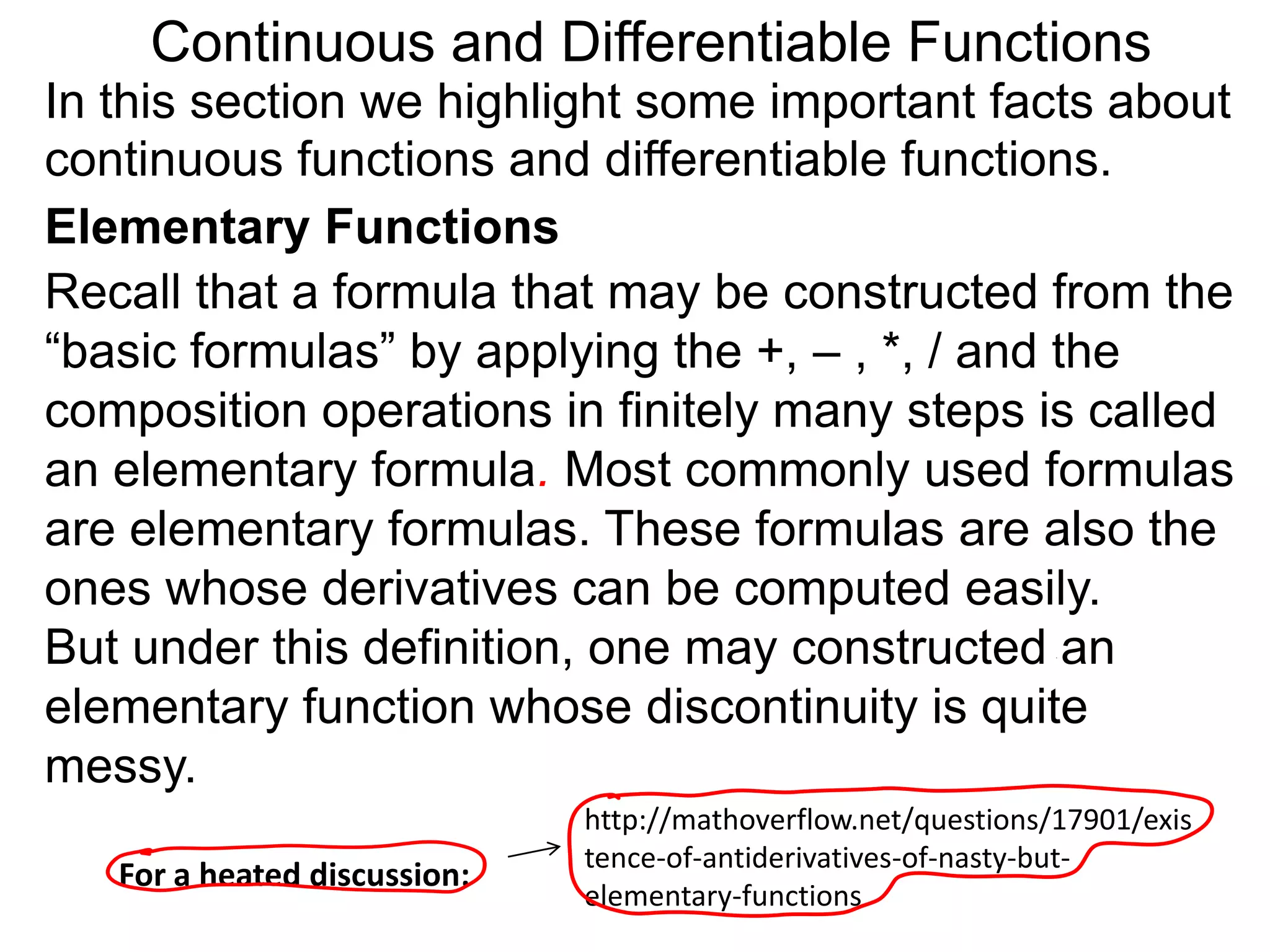
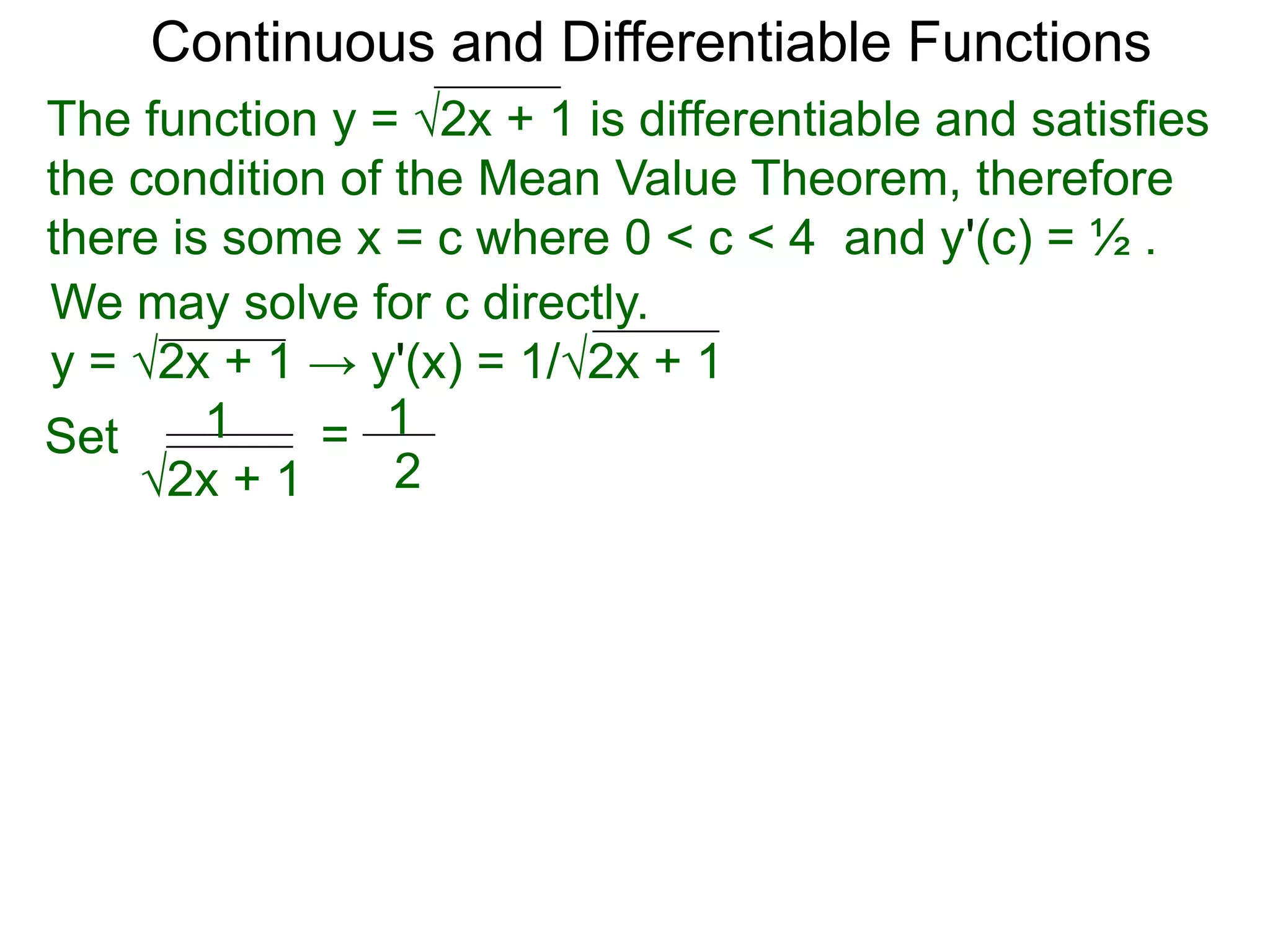
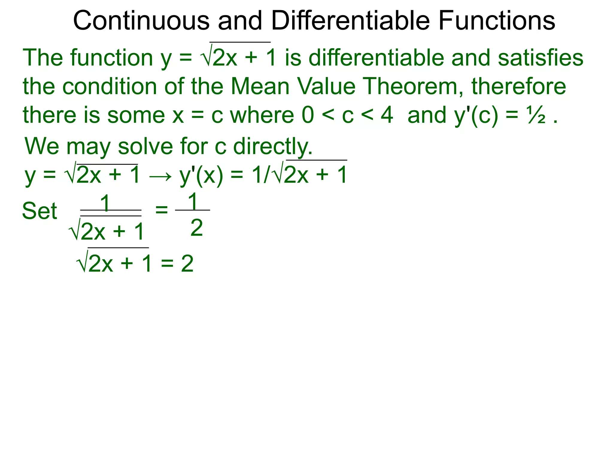
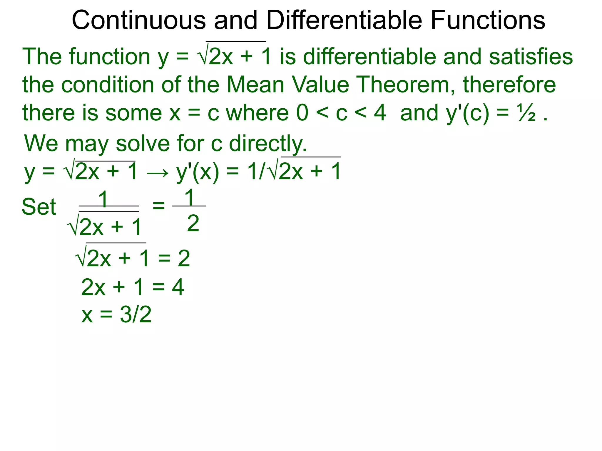
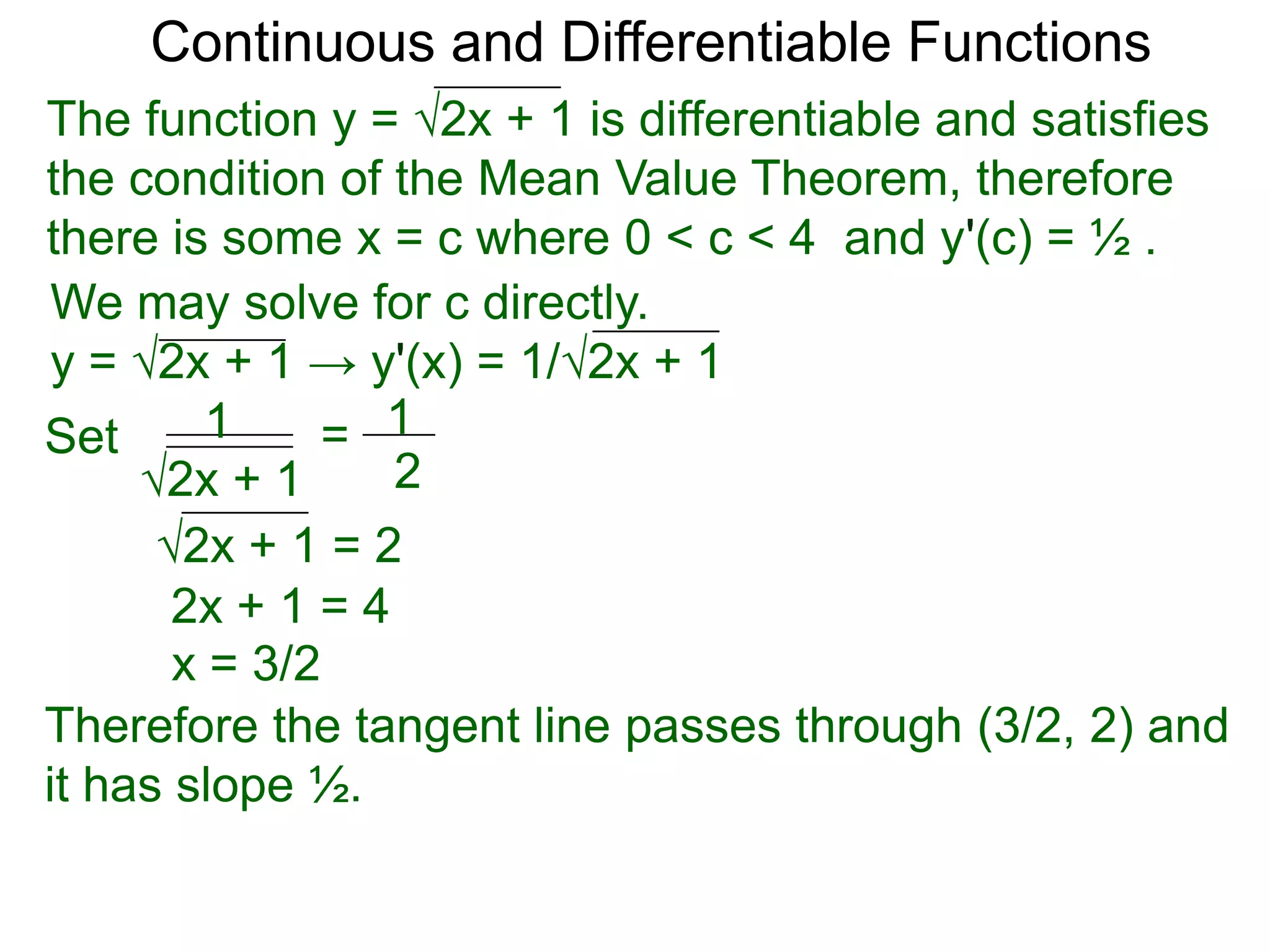
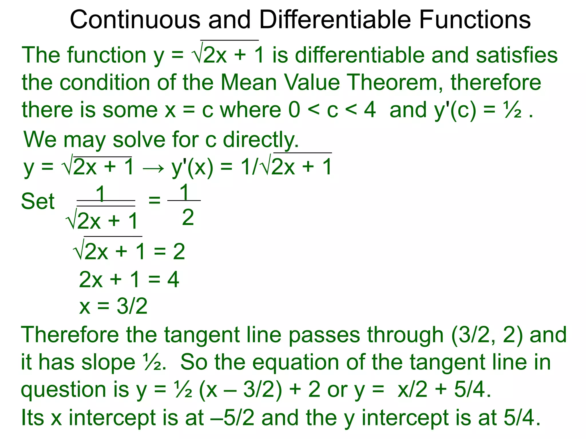
The document discusses continuous and differentiable functions. It defines elementary functions as those constructed using basic operations like addition and multiplication. Continuous functions over a closed interval are bounded and have absolute maximum and minimum values. The Intermediate Value Theorem states that a continuous function takes on all values between its minimum and maximum. Differentiable functions are continuous. Rolle's Theorem says that if a differentiable function is equal at the endpoints of an interval, its derivative is zero somewhere in between.

![Continuous and Differentiable Functions
Continuous Functions
There are two important facts about continuous
functions.
I. Intermediate Value Theorem
Let f(x) be a continuous function defined over the
closed interval [a, b] such that f(a) < f(b),](https://image.slidesharecdn.com/4-5continuousfunctionsanddifferentiablefunctions-120508095708-phpapp01/75/4-5-continuous-functions-and-differentiable-functions-13-2048.jpg)
![Continuous and Differentiable Functions
Continuous Functions
There are two important facts about continuous
functions.
I. Intermediate Value Theorem
Let f(x) be a continuous function defined over the
closed interval [a, b] such that f(a) < f(b),
f(b)
f(a)
a b](https://image.slidesharecdn.com/4-5continuousfunctionsanddifferentiablefunctions-120508095708-phpapp01/75/4-5-continuous-functions-and-differentiable-functions-14-2048.jpg)
![Continuous and Differentiable Functions
Continuous Functions
There are two important facts about continuous
functions.
I. Intermediate Value Theorem
Let f(x) be a continuous function defined over the
closed interval [a, b] such that f(a) < f(b),
let m be any number where f(a) < m < f(b),
f(b)
m
f(a)
a b](https://image.slidesharecdn.com/4-5continuousfunctionsanddifferentiablefunctions-120508095708-phpapp01/75/4-5-continuous-functions-and-differentiable-functions-15-2048.jpg)
![Continuous and Differentiable Functions
Continuous Functions
There are two important facts about continuous
functions.
I. Intermediate Value Theorem
Let f(x) be a continuous function defined over the
closed interval [a, b] such that f(a) < f(b),
let m be any number where f(a) < m < f(b),
then there exists at least
one c, i.e. one or more, f(b)
where a < c < b,
m
f(a)
a c b](https://image.slidesharecdn.com/4-5continuousfunctionsanddifferentiablefunctions-120508095708-phpapp01/75/4-5-continuous-functions-and-differentiable-functions-16-2048.jpg)
![Continuous and Differentiable Functions
Continuous Functions
There are two important facts about continuous
functions.
I. Intermediate Value Theorem
Let f(x) be a continuous function defined over the
closed interval [a, b] such that f(a) < f(b),
let m be any number where f(a) < m < f(b),
then there exists at least
one c, i.e. one or more, f(b)
where a < c < b,
m
and that f(c) = m.
f(a)
a c b](https://image.slidesharecdn.com/4-5continuousfunctionsanddifferentiablefunctions-120508095708-phpapp01/75/4-5-continuous-functions-and-differentiable-functions-17-2048.jpg)
![Continuous and Differentiable Functions
Continuous Functions
There are two important facts about continuous
functions.
I. Intermediate Value Theorem
Let f(x) be a continuous function defined over the
closed interval [a, b] such that f(a) < f(b),
let m be any number where f(a) < m < f(b),
then there exists at least other c’s
one c, i.e. one or more, f(b)
where a < c < b,
m
and that f(c) = m.
f(a)
a c b](https://image.slidesharecdn.com/4-5continuousfunctionsanddifferentiablefunctions-120508095708-phpapp01/75/4-5-continuous-functions-and-differentiable-functions-18-2048.jpg)
![Continuous and Differentiable Functions
Continuous Functions
There are two important facts about continuous
functions.
I. Intermediate Value Theorem
Let f(x) be a continuous function defined over the
closed interval [a, b] such that f(a) < f(b),
let m be any number where f(a) < m < f(b),
then there exists at least other c’s
one c, i.e. one or more, f(b)
where a < c < b,
m
and that f(c) = m.
We omit the proof here. f(a)
Here is a link to its proof.
http://en.wikipedia.org/wiki/Intermediate a c b
_value_theorem](https://image.slidesharecdn.com/4-5continuousfunctionsanddifferentiablefunctions-120508095708-phpapp01/75/4-5-continuous-functions-and-differentiable-functions-19-2048.jpg)

![Continuous and Differentiable Functions
Remarks
I. Similarly, if f(a) > f(b) then there is some c with
a < c < b such that f(c) = m for f(a) > m > f(b).
II. If the condition is f(a) ≤ m ≤ f(b) then the
conclusion is a ≤ c ≤ b.
One important application for this theorem is the
existence of roots.
(Bozano’s Theorem) Let y = f(x) be a continuous
function over the closed interval [a, b], then there
exists at least one c where a < c < b with f(c) = 0
if the signs of f(a) and f(b) are different.](https://image.slidesharecdn.com/4-5continuousfunctionsanddifferentiablefunctions-120508095708-phpapp01/75/4-5-continuous-functions-and-differentiable-functions-23-2048.jpg)
![Continuous and Differentiable Functions
Remarks
I. Similarly, if f(a) > f(b) then there is some c with
a < c < b such that f(c) = m for f(a) > m > f(b).
II. If the condition is f(a) ≤ m ≤ f(b) then the
conclusion is a ≤ c ≤ b.
One important application for this theorem is the
existence of roots.
(Bozano’s Theorem) Let y = f(x) be a continuous
function over the closed interval [a, b], then there
exists at least one c where a < c < b with f(c) = 0
if the signs of f(a) and f(b) are different.
With this theorem, we conclude that f(x) = x3 – 3x2 – 5
has a root between 2 < x < 5, as in 3.6 Example B,
because f(2) and f(5) have opposite signs.](https://image.slidesharecdn.com/4-5continuousfunctionsanddifferentiablefunctions-120508095708-phpapp01/75/4-5-continuous-functions-and-differentiable-functions-24-2048.jpg)
![Continuous and Differentiable Functions
The other important fact about continuous functions
is the existence of extrema over a closed interval.
II. Extrema Theorem for Continuous Functions
Let y = f(x) be a continuous function defined over a
closed interval V = [a, b], then both the absolute max.
and the absolute min. exist in V.](https://image.slidesharecdn.com/4-5continuousfunctionsanddifferentiablefunctions-120508095708-phpapp01/75/4-5-continuous-functions-and-differentiable-functions-27-2048.jpg)
![Continuous and Differentiable Functions
The other important fact about continuous functions
is the existence of extrema over a closed interval.
II. Extrema Theorem for Continuous Functions
Let y = f(x) be a continuous function defined over a
closed interval V = [a, b], then both the absolute max.
and the absolute min. exist in V.
In particular if M is the maximum and m is the minimum,
then m ≤ f(x) ≤ M for every x in the interval [a, b].](https://image.slidesharecdn.com/4-5continuousfunctionsanddifferentiablefunctions-120508095708-phpapp01/75/4-5-continuous-functions-and-differentiable-functions-28-2048.jpg)
![Continuous and Differentiable Functions
The other important fact about continuous functions
is the existence of extrema over a closed interval.
II. Extrema Theorem for Continuous Functions
Let y = f(x) be a continuous function defined over a
closed interval V = [a, b], then both the absolute max.
and the absolute min. exist in V.
In particular if M is the maximum and m is the minimum,
then m ≤ f(x) ≤ M for every x in the interval [a, b].
So a continuous function defined over a closed
interval V is always bounded.](https://image.slidesharecdn.com/4-5continuousfunctionsanddifferentiablefunctions-120508095708-phpapp01/75/4-5-continuous-functions-and-differentiable-functions-29-2048.jpg)
![Continuous and Differentiable Functions
The other important fact about continuous functions
is the existence of extrema over a closed interval.
II. Extrema Theorem for Continuous Functions
Let y = f(x) be a continuous function defined over a
closed interval V = [a, b], then both the absolute max.
and the absolute min. exist in V.
In particular if M is the maximum and m is the minimum,
then m ≤ f(x) ≤ M for every x in the interval [a, b].
So a continuous function defined over a closed
interval V is always bounded.
Corollary. Let y = f(x) be an elementary function
defined over a closed interval V = [a, b], then f(x) is
continuous over [a, b], hence both the absolute max.
and the absolute min. exist in V.](https://image.slidesharecdn.com/4-5continuousfunctionsanddifferentiablefunctions-120508095708-phpapp01/75/4-5-continuous-functions-and-differentiable-functions-30-2048.jpg)
![Continuous and Differentiable Functions
Rolle’s Theorem
Let f(x) be a differentiable function defined over the
closed interval [a, b] with a < b and that f(a) = f(b),](https://image.slidesharecdn.com/4-5continuousfunctionsanddifferentiablefunctions-120508095708-phpapp01/75/4-5-continuous-functions-and-differentiable-functions-38-2048.jpg)
![Continuous and Differentiable Functions
Rolle’s Theorem
Let f(x) be a differentiable function defined over the
closed interval [a, b] with a < b and that f(a) = f(b),
f(a)=f(b)
x
a c b x](https://image.slidesharecdn.com/4-5continuousfunctionsanddifferentiablefunctions-120508095708-phpapp01/75/4-5-continuous-functions-and-differentiable-functions-39-2048.jpg)
![Continuous and Differentiable Functions
Rolle’s Theorem
Let f(x) be a differentiable function defined over the
closed interval [a, b] with a < b and that f(a) = f(b),
then there is at least one c where a < c < b
such that f'(c) = 0. other c’s
f'(c) = 0
f(a)=f(b)
x
a c b x](https://image.slidesharecdn.com/4-5continuousfunctionsanddifferentiablefunctions-120508095708-phpapp01/75/4-5-continuous-functions-and-differentiable-functions-40-2048.jpg)
![Continuous and Differentiable Functions
Rolle’s Theorem
Let f(x) be a differentiable function defined over the
closed interval [a, b] with a < b and that f(a) = f(b),
then there is at least one c where a < c < b
such that f'(c) = 0. other c’s
Proof. Consider the following f'(c) = 0
two cases.
f(a)=f(b)
x
a c b x](https://image.slidesharecdn.com/4-5continuousfunctionsanddifferentiablefunctions-120508095708-phpapp01/75/4-5-continuous-functions-and-differentiable-functions-41-2048.jpg)
![Continuous and Differentiable Functions
Rolle’s Theorem
Let f(x) be a differentiable function defined over the
closed interval [a, b] with a < b and that f(a) = f(b),
then there is at least one c where a < c < b
such that f'(c) = 0. other c’s
Proof. Consider the following f'(c) = 0
two cases.
1. The function f(x) is a f(a)=f(b)
constant function, i.e. x
a c b x
f(x) = f(a) = k, then f'(x) = 0](https://image.slidesharecdn.com/4-5continuousfunctionsanddifferentiablefunctions-120508095708-phpapp01/75/4-5-continuous-functions-and-differentiable-functions-42-2048.jpg)
![Continuous and Differentiable Functions
Rolle’s Theorem
Let f(x) be a differentiable function defined over the
closed interval [a, b] with a < b and that f(a) = f(b),
then there is at least one c where a < c < b
such that f'(c) = 0. other c’s
Proof. Consider the following f'(c) = 0
two cases.
1. The function f(x) is a f(a)=f(b)
constant function, i.e. x
a c b x
f(x) = f(a) = k, then f'(x) = 0.
Any number c where a < c < b would satisfy f'(c) = 0.](https://image.slidesharecdn.com/4-5continuousfunctionsanddifferentiablefunctions-120508095708-phpapp01/75/4-5-continuous-functions-and-differentiable-functions-43-2048.jpg)
![Continuous and Differentiable Functions
Rolle’s Theorem
Let f(x) be a differentiable function defined over the
closed interval [a, b] with a < b and that f(a) = f(b),
then there is at least one c where a < c < b
such that f'(c) = 0. other c’s
Proof. Consider the following f'(c) = 0
two cases.
1. The function f(x) is a f(a)=f(b)
constant function, i.e. x
a c b x
f(x) = f(a) = k, then f'(x) = 0
Any number c where a < c < b would satisfy f'(c) = 0.
2. If the function f(x) is not a constant function,
then there exists an extremum c between a and b, with
f(c) ≠ f(a) and f(c) ≠ (b) and we must have f'(c) = 0.](https://image.slidesharecdn.com/4-5continuousfunctionsanddifferentiablefunctions-120508095708-phpapp01/75/4-5-continuous-functions-and-differentiable-functions-44-2048.jpg)
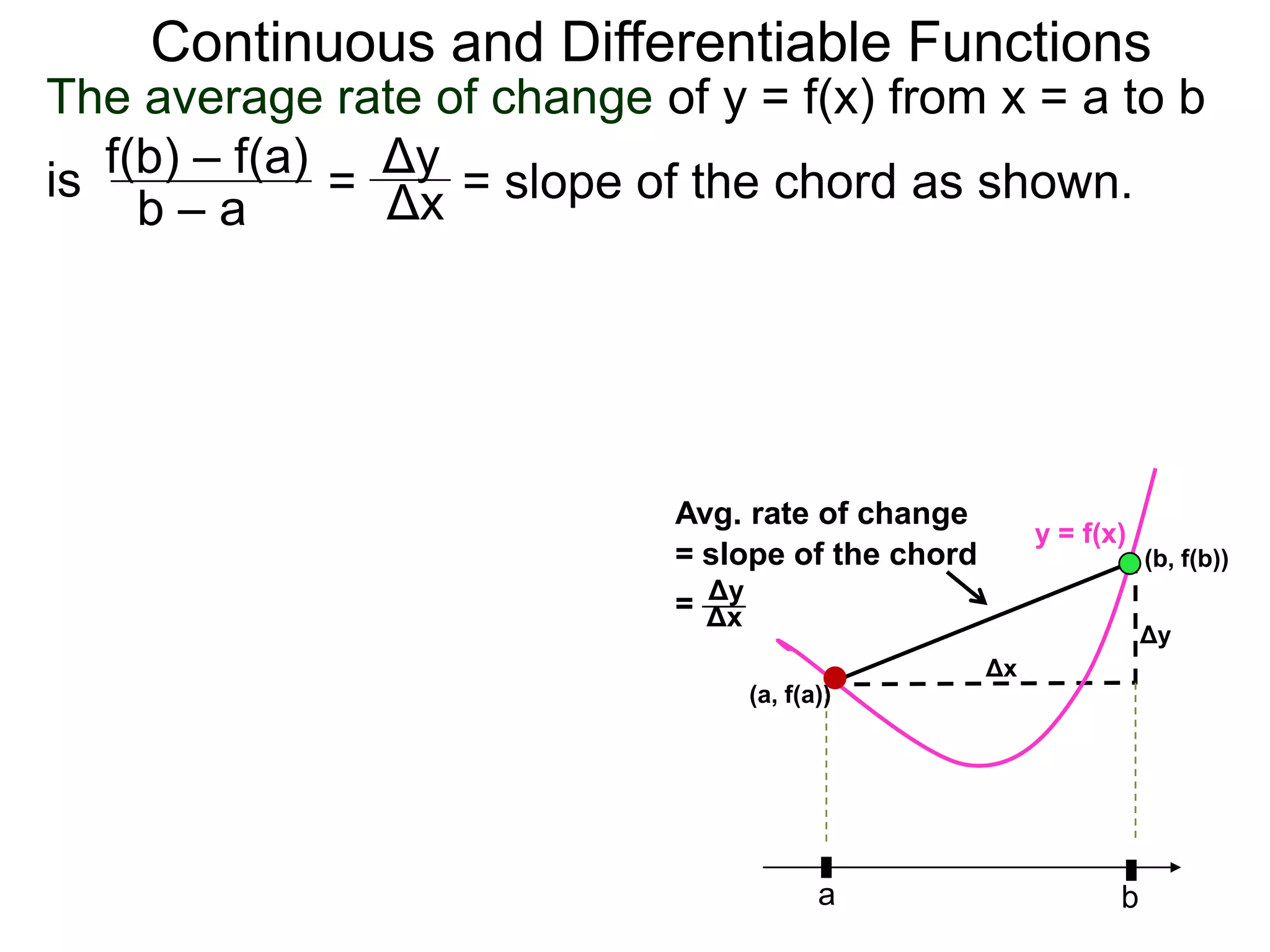
![Continuous and Differentiable Functions
The average rate of change of y = f(x) from x = a to b
is f(b) – f(a) = Δy = slope of the chord as shown.
Δx
b–a
The graph y = f(x) is the rotation of the graph of some
function y = g(x) defined over some interval [A, B]
Avg. rate of change
y = g(x) y = f(x)
= slope of the chord (b, f(b))
g(A) = g(B) Δy
= Δx
(A, g(A)) (B, g(B)) Δy
Δx
(a, f(a))
Rotate
A C B a b](https://image.slidesharecdn.com/4-5continuousfunctionsanddifferentiablefunctions-120508095708-phpapp01/75/4-5-continuous-functions-and-differentiable-functions-46-2048.jpg)
![Continuous and Differentiable Functions
The average rate of change of y = f(x) from x = a to b
is f(b) – f(a) = Δy = slope of the chord as shown.
Δx
b–a
The graph y = f(x) is the rotation of the graph of some
function y = g(x) defined over some interval [A, B]
with g(A) = g(B) with the rotation taking
(A,g(A)) to (a, f(a)) and (B,g(B)) to (b, f(b)) as shown.
Avg. rate of change
y = g(x) y = f(x)
= slope of the chord (b, f(b))
g(A) = g(B) Δy
= Δx
(A, g(A)) (B, g(B)) Δy
Δx
(a, f(a))
Rotate
A C B a b](https://image.slidesharecdn.com/4-5continuousfunctionsanddifferentiablefunctions-120508095708-phpapp01/75/4-5-continuous-functions-and-differentiable-functions-47-2048.jpg)
![Continuous and Differentiable Functions
If in addition y = g(x) is differentiable over an interval
that contains [A, B], then Rolle’s Theorem implies the
existence of at least one C where A < C < B such that
the tangent line at (C, g(C)) is a horizontal.
y = f(x)
Rolle’s Theorem
y = g(x) (b, f(b))
g(A) = g(B)
(A, g(A)) (B, g(B))
(a, f(a))
There exists a C
where g'(C) = 0 Rotate
A C B a b](https://image.slidesharecdn.com/4-5continuousfunctionsanddifferentiablefunctions-120508095708-phpapp01/75/4-5-continuous-functions-and-differentiable-functions-48-2048.jpg)
![Continuous and Differentiable Functions
If in addition y = g(x) is differentiable over an interval
that contains [A, B], then Rolle’s Theorem implies the
existence of at least one C where A < C < B such that
the tangent line at (C, g(C)) is a horizontal. Under the
rotation this horizontal line rotates into a tangent line
that is parallel to the chord from (a, f(a)) to (b, f(b))
y = f(x)
Rolle’s Theorem
y = g(x) (b, f(b))
g(A) = g(B)
(A, g(A)) (B, g(B))
(a, f(a))
There exists a C There exists a C where
where g'(C) = 0 Rotate f '(C) = Avg. rate of change
A C B a b](https://image.slidesharecdn.com/4-5continuousfunctionsanddifferentiablefunctions-120508095708-phpapp01/75/4-5-continuous-functions-and-differentiable-functions-49-2048.jpg)
![Continuous and Differentiable Functions
If in addition y = g(x) is differentiable over an interval
that contains [A, B], then Rolle’s Theorem implies the
existence of at least one C where A < C < B such that
the tangent line at (C, g(C)) is a horizontal. Under the
rotation this horizontal line rotates into a tangent line
that is parallel to the chord from (a, f(a)) to (b, f(b))
which gives us the Mean Value Theorem. y = f(x)
Rolle’s Theorem Mean Value Theorem
y = g(x) (b, f(b))
g(A) = g(B)
(A, g(A)) (B, g(B))
(a, f(a))
There exists a C There exists a C where
where g'(C) = 0 Rotate f '(C) = Avg. rate of change
A C B a b](https://image.slidesharecdn.com/4-5continuousfunctionsanddifferentiablefunctions-120508095708-phpapp01/75/4-5-continuous-functions-and-differentiable-functions-50-2048.jpg)
![Continuous and Differentiable Functions
Mean Value Theorem
Let y = f(x) be a differentiable function over an interval
that contains [a, b], then there is at least one c where
a < c < b such that y = f(x)
f '(c) = f(b) – f(a) . slope = Avg. rate of change (b, f(b))
b–a =
f(b) – f(a)
b–a .
(a, f(a))
a c b
There exists a c where
f(b) – f(a)
f '(c) = Avg. rate of change =
b–a .](https://image.slidesharecdn.com/4-5continuousfunctionsanddifferentiablefunctions-120508095708-phpapp01/75/4-5-continuous-functions-and-differentiable-functions-51-2048.jpg)
![Continuous and Differentiable Functions
Mean Value Theorem
Let y = f(x) be a differentiable function over an interval
that contains [a, b], then there is at least one c where
a < c < b such that y = f(x)
f '(c) = f(b) – f(a) . slope = Avg. rate of change (b, f(b))
b–a =
f(b) – f(a)
b–a .
Remarks
1. The precise condition
for the theorem is that (a, f(a))
f(x) is continuous in [a, b],
and differentiable in (a, b).
The condition above is
stronger but is sufficient a c b
for our purposes. There exists a c where
f(b) – f(a)
f '(c) = Avg. rate of change =
b–a .](https://image.slidesharecdn.com/4-5continuousfunctionsanddifferentiablefunctions-120508095708-phpapp01/75/4-5-continuous-functions-and-differentiable-functions-52-2048.jpg)
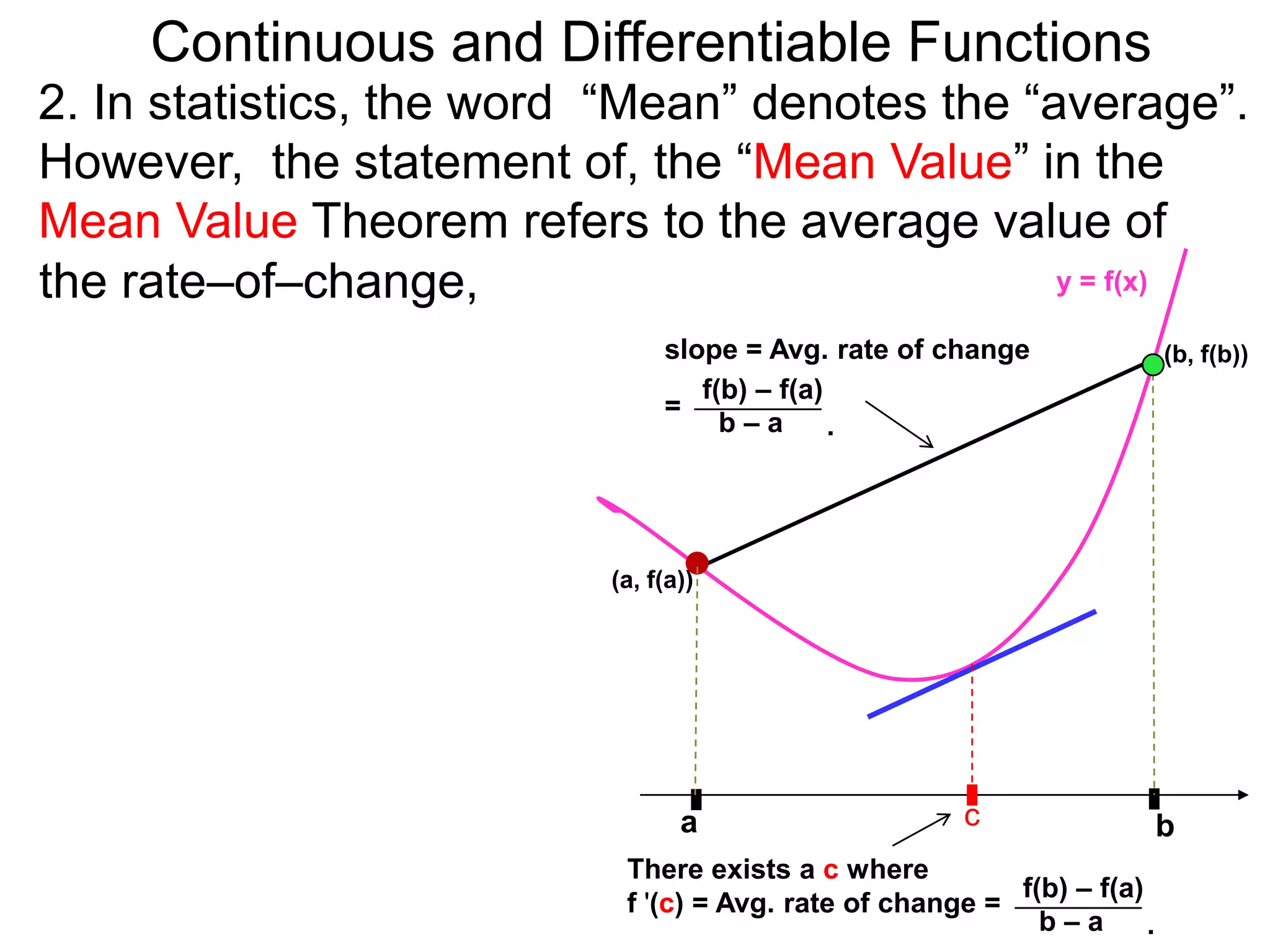
![Continuous and Differentiable Functions
2. In statistics, the word “Mean” denotes the “average”.
However, the statement of, the “Mean Value” in the
Mean Value Theorem refers to the average value of
the rate–of–change, y = f(x)
not the “mean value” slope = Avg. rate of change (b, f(b))
f(b) – f(a)
or the average value of =
b–a .
the function f(x) over the
interval [a, b].
(a, f(a))
a c b
There exists a c where
f(b) – f(a)
f '(c) = Avg. rate of change =
b–a .](https://image.slidesharecdn.com/4-5continuousfunctionsanddifferentiablefunctions-120508095708-phpapp01/75/4-5-continuous-functions-and-differentiable-functions-54-2048.jpg)
![Continuous and Differentiable Functions
2. In statistics, the word “Mean” denotes the “average”.
However, the statement of, the “Mean Value” in the
Mean Value Theorem refers to the average value of
the rate–of–change, y = f(x)
not the “mean value” slope = Avg. rate of change (b, f(b))
f(b) – f(a)
or the average value of =
b–a .
the function f(x) over the
interval [a, b].
The average value of (a, f(a))
the function f(x) over the
interval [a, b] is defined
by integrals which are
c
our next topics. a b
There exists a c where
f(b) – f(a)
f '(c) = Avg. rate of change =
b–a .](https://image.slidesharecdn.com/4-5continuousfunctionsanddifferentiablefunctions-120508095708-phpapp01/75/4-5-continuous-functions-and-differentiable-functions-55-2048.jpg)


![Limits and continuity[1]](https://cdn.slidesharecdn.com/ss_thumbnails/limitsandcontinuity1-110816105053-phpapp01-thumbnail.jpg?width=640&height=640&fit=bounds)


