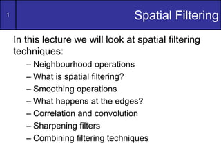
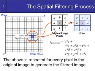
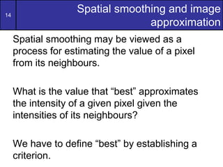
1. Spatial filtering techniques include neighbourhood operations, smoothing filters, sharpening filters, and combining filtering techniques. Neighbourhood operations operate on pixels surrounding a central pixel. 2. Simple neighbourhood operations include minimum, maximum, and median filters. Smoothing filters average pixel values in a neighbourhood to reduce noise while preserving edges. 3. Convolution and correlation are similar operations that involve multiplying a filter kernel with pixels in an image neighbourhood. Convolution involves flipping the filter kernel before multiplication.

1. 1 Spatial Filtering
In this lecture we will look at spatial filtering
techniques:
– Neighbourhood operations
– What is spatial filtering?
– Smoothing operations
– What happens at the edges?
– Correlation and convolution
– Sharpening filters
– Combining filtering techniques

2. 2 Neighbourhood Operations
Neighbourhood operations simply operate
on a larger neighbourhood of pixels than
point operations
Neighbourhoods are
mostly a rectangle
around a central pixel
Any size rectangle
and any shape filter
are possible
Origin x
y Image f (x, y)
(x, y)
Neighbourhood

3. 3 Simple Neighbourhood Operations
Some simple neighbourhood operations
include:
– Min: Set the pixel value to the minimum in
the neighbourhood
– Max: Set the pixel value to the maximum in
the neighbourhood
– Median: The median value of a set of
numbers is the midpoint value in that set (e.g.
from the set [1, 7, 15, 18, 24] 15 is the
median). Sometimes the median works better
than the average

4. 4
Simple Neighbourhood Operations
Example
123 127 128 119 115 130
140 145 148 153 167 172
133 154 183 192 194 191
194 199 207 210 198 195
164 170 175 162 173 151
Original Image x
y
Enhanced Image x
y

5. 5 The Spatial Filtering Process
r s t
u v w
x y z
Origin x
y Image f (x, y)
eprocessed = v*e +
r*a + s*b + t*c +
u*d + w*f +
x*g + y*h + z*i
Filter
Simple 3*3
Neighbourhood
e 3*3 Filter
a b c
d e f
g h i
Original Image
Pixels
*
The above is repeated for every pixel in the
original image to generate the filtered image

6. 6

7. 7 Spatial Filtering: Equation Form


 




a
a
s
b
b
t
t
y
s
x
f
t
s
w
y
x
g )
,
(
)
,
(
)
,
(
Filtering can be given
in equation form as
shown above
Notations are based
on the image shown
to the left

8. 8 Smoothing Spatial Filters
One of the simplest spatial filtering
operations we can perform is a smoothing
operation
– Simply average all of the pixels in a
neighbourhood around a central value
– Especially useful
in removing noise
from images
– Also useful for
highlighting gross
detail
1/9
1/9
1/9
1/9
1/9
1/9
1/9
1/9
1/9
Simple
averaging
filter

9. 9 Smoothing Spatial Filtering
1/9
1/9
1/9
1/9
1/9
1/9
1/9
1/9
1/9
Origin x
y Image f (x, y)
e = 1/9*106 +
1/9*104 + 1/9*100 + 1/9*108 +
1/9*99 + 1/9*98 +
1/9*95 + 1/9*90 + 1/9*85
= 98.3333
Filter
Simple 3*3
Neighbourhood
106
104
99
95
100 108
98
90 85
1/9
1/9
1/9
1/9
1/9
1/9
1/9
1/9
1/9
3*3 Smoothing
Filter
104 100 108
99 106 98
95 90 85
Original Image
Pixels
*
The above is repeated for every pixel in the original image to
generate the smoothed image.

10. 10 Image Smoothing Example
The image at the top left
is an original image of
size 500*500 pixels
The subsequent images
show the image after
filtering with an averaging
filter of increasing sizes
– 3, 5, 9, 15 and 35
Notice how detail begins
to disappear

11. 11 Weighted Smoothing Filters
More effective smoothing filters can be
generated by allowing different pixels in the
neighbourhood different weights in the
averaging function
– Pixels closer to the
central pixel are more
important
– Often referred to as a
weighted averaging
1/16
2/16
1/16
2/16
4/16
2/16
1/16
2/16
1/16
Weighted
averaging filter

12. 12 Another Smoothing Example
By smoothing the original image we get rid
of lots of the finer detail which leaves only
the gross features for thresholding
Original Image Smoothed Image Thresholded Image

13. 13
Averaging Filter Vs. Median Filter
Example
Filtering is often used to remove noise from
images
Sometimes a median filter works better than
an averaging filter
Original Image
With Noise
Image After
Averaging Filter
Image After
Median Filter

14. 14
Spatial smoothing and image
approximation
Spatial smoothing may be viewed as a
process for estimating the value of a pixel
from its neighbours.
What is the value that “best” approximates
the intensity of a given pixel given the
intensities of its neighbours?
We have to define “best” by establishing a
criterion.

15. 15
Spatial smoothing and image
approximation (cont...)
 
2
1
( )
N
i
E x i m

 
  
2
1
argmin ( )
N
m i
m x i m

 
  
 
 

0
E
m



 
1
2 ( ) 0
N
i
x i m

   
 1 1
( )
N N
i i
x i m
 
 
 
1
( )
N
i
x i Nm

 

1
1
( )
N
i
m x i
N 
  
A standard criterion is the the sum of
squares differences.
The average value

16. 16
Spatial smoothing and image
approximation (cont...)
1
( )
N
i
E x i m

 
 1
argmin ( )
N
m i
m x i m

 
  
 
 

0
E
m



 
1
( ) 0,
N
i
sgn x i m

   

1 0
( ) 0 0
1 0
x
sign x x
x



 

 

Another criterion is the the sum of absolute
differences.
There must be equal in quantity positive and negative values.
median{ ( )}
m x i


17. 17
Spatial smoothing and image
approximation (cont...)
– It works well for impulse noise (e.g. salt and
pepper).
– It requires sorting of the image values.
– It preserves the edges better than an average
filter in the case of impulse noise.
– It is robust to impulse noise at 50%.

18. 18
Spatial smoothing and image
approximation (cont...)
Example x[n] 1 1 1 1 1 2 2 2 2 2
Impulse
noise
x[n] 1 3 1 1 1 2 3 2 2 3
Median
(N=3) x[n] - 1 1 1 1 2 2 2 2 -
Average
(N=3)
x[n] - 1.7 1.7 1 1.3 2 2.3 2.3 2.2 -
edge
The edge is smoothed

19. 19 Correlation & Convolution
The filtering we have been talking about so
far is referred to as correlation with the filter
itself referred to as the correlation kernel
Convolution is a similar operation, with just
one subtle difference
For symmetric filters it makes no difference.
eprocessed = v*e +
z*a + y*b + x*c +
w*d + u*e +
t*f + s*g + r*h
r s t
u v w
x y z
Filter
a b c
d e e
f g h
Original Image
Pixels
*

20. 20

21. 21 What is Convolution?
• Convolution provides a way of `multiplying
together' two arrays of numbers, generally of
different sizes, but of the same
dimensionality, to produce a third array of
numbers of the same dimensionality.
• It can be mathematically represented as two
ways:
– Mask convolved with an image
g(x,y) = h(x,y) * f(x,y)
– Image convolved with mask
g(x,y) = f(x,y) * h(x,y), here, Image is f(x,y) and Mask is h(x,y)
• There are two ways to represent this because the
convolution operator(*) is commutative.

22. 22 What is Mask?
• Mask is also a signal & it can be
represented by a two dimensional matrix.
• The mask is usually of the order of 1x1,
3x3, 5x5, 7x7.
• A mask should always be in odd number,
because other wise you cannot find the mid
(center) of the mask.
• Center of the mask is used in convolution.

23. 23 How to Perform Convolution?
• In order to perform convolution on an
image, following steps should be taken:
– Flip the mask (horizontally and vertically) only
once
– Perform the correlation of mask with image
by following steps:
• Slide the mask onto the image.
• Multiply the corresponding elements & then add
these.
• Repeat this procedure until all values of the image
have been computed.

24. 24
1 -1 -1
1 2 -1
1 1 1
2 2 2 3
2 1 3 3
2 2 1 2
1 3 2 2
Don’t rotate use it directly
correlation kernel, ω
Input Image f
Correlation

25. 25
3
2
1
2
2
1
3
2
3
2
2
1
2
2
3
2 5
3
2
1
2
2
1
3
2
3
2
2
1
2
2
3
2
1
2
1
-2
4
1
-1
-1
1
1
1
1
-1
2
1
-1
-1
1
Input Image, f
output
Image, g
Correlation

26. 26
3
2
1
2
2
1
3
2
3
2
2
1
2
2
3
2 10
5
3
2
1
2
2
1
3
2
3
2
2
1
2
2
3
2
3
1
2
-2
4
2
-1
-1
1
1
1
1
-1
2
1
-1
-1
1
Input Image, f
output
Image, g
Correlation

27. 27
3
2
1
2
2
1
3
2
3
2
2
1
2
2
3
2 10 10
5
3
2
1
2
2
1
3
2
3
2
2
1
2
2
3
2
3
3
1
-3
4
2
-1
-1
1
1
1
1
-1
2
1
-1
-1
1
Input Image, f
output
Image, g
Correlation

28. 28
3
2
1
2
2
1
3
2
3
2
2
1
2
2
3
2 10 10 15
5
3
2
1
2
2
1
3
2
3
2
2
1
2
2
3
2
1
3
3
-1
6
2
-1
-1
1
1
1
1
-1
2
1
-1
-1
1
Input Image, f
output
Image, g
Correlation

29. 29
3
2
1
2
2
1
3
2
3
2
2
1
2
2
3
2 10 10
3
15
5
3
2
1
2
2
1
3
2
3
2
2
1
2
2
3
2
2
2
1
-1
4
1
-2
-2
1
1
1
1
-1
2
1
-1
-1
1
Input Image, f
output
Image, g
Correlation

30. 30
3
2
1
2
2
1
3
2
3
2
2
1
2
2
3
2
4
10 10
3
15
5
3
2
1
2
2
1
3
2
3
2
2
1
2
2
3
2
1
2
2
-3
2
2
-2
-2
2
1
1
1
-1
2
1
-1
-1
1
Input Image, f
output
Image, g
Correlation

31. 31
4
11
4
10
4
4
6
10
11
3
5
-5
9
7
15
5
Final output Image “g”
Correlation

32. 32
Convolution
1 -1 -1
1 2 -1
1 1 1
2 2 2 3
2 1 3 3
2 2 1 2
1 3 2 2
Rotate 180o
1
-1
-1
1
2
-1
1
1
1
Convolution kernel, ω Input Image, f

33. 33 Convolution
Input Image, f
3
2
1
2
2
1
3
2
3
2
2
1
2
2
3
2 5
3
2
1
2
2
1
3
2
3
2
2
1
2
2
3
2
1
-2
-1
2
4
-1
1
1
1
1
-1
-1
1
2
-1
1
1
1
Output
Image, g

34. 34
3
2
1
2
2
1
3
2
3
2
2
1
2
2
3
2 4
5
3
2
1
2
2
1
3
2
3
2
2
1
2
2
3
2
3
-1
-2
2
4
-2
1
1
1
1
-1
-1
1
2
-1
1
1
1
Input Image, f
Output
Image, g
Convolution

35. 35
3
2
1
2
2
1
3
2
3
2
2
1
2
2
3
2 4 4
5
3
2
1
2
2
1
3
2
3
2
2
1
2
2
3
2
3
-3
-1
3
4
-2
1
1
1
1
-1
-1
1
2
-1
1
1
1
Input Image, f
Output
Image, g
Convolution

36. 36
3
2
1
2
2
1
3
2
3
2
2
1
2
2
3
2 4 4 -2
5
3
2
1
2
2
1
3
2
3
2
2
1
2
2
3
2
1
-3
-3
1
6
-2
1
1
1
1
-1
-1
1
2
-1
1
1
1
Input Image, f
Output
Image, g
Convolution

37. 37
3
2
1
2
2
1
3
2
3
2
2
1
2
2
3
2 4 4
9
-2
5
3
2
1
2
2
1
3
2
3
2
2
1
2
2
3
2
2
-2
-1
1
4
-1
2
2
1
1
-1
-1
1
2
-1
1
1
1
Input Image, f
Output
Image, g
Convolution

38. 38
3
2
1
2
2
1
3
2
3
2
2
1
2
2
3
2
6
4 4
9
-2
5
3
2
1
2
2
1
3
2
3
2
2
1
2
2
3
2
1
-2
-2
3
2
-2
2
2
2
1
-1
-1
1
2
-1
1
1
1
Input Image, f
Output
Image, g
Convolution

39. 39
12
7
6
4
8
6
14
4
5
9
5
9
5
11
-2
5
Final output Image, g
Convolution

40. 40 Strange Things Happen At The Edges!
Origin x
y Image f (x, y)
e
e
e
e
At the edges of an image we are missing
pixels to form a neighbourhood
e e
e

41. 41
Strange Things Happen At The Edges!
(cont…)
There are a few approaches to dealing with
missing edge pixels:
– Omit missing pixels
• Only works with some filters
• Can add extra code and slow down processing
– Pad the image
• Typically with either all white or all black pixels
– Replicate border pixels
– Truncate the image
– Allow pixels wrap around the image
• Can cause some strange image artefacts

42. 42

43. 43
Strange Things Happen At The Edges!
(cont…)
Original
Image
Filtered Image:
Zero Padding
Filtered Image:
Replicate Edge Pixels
Filtered Image:
Wrap Around Edge Pixels

44. 44 Spatial Filter
• A spatial filter is an image operation
where each pixel value I(u; v) is changed
by a function of the intensities of pixels in
a neighborhood of (u; v).
• It involves moving the filter mask from
point to point in an image.
• At each point (x,y), the response of the
filter at that point is calculated using a
predefined relationship.

45. 45 Example (Mean Filtering)
10 12 11 2 3 15
12 12 1 1 2 1
2 3 5 6 4 5
1 4 51 12 14 12
12 10 12 13 13 10
23 1 10 12 12 12
1/9 1/9 1/9
1/9 1/9 1/9
1/9 1/9 1/9
Input image I
Filter H of 3x3 size
• Consider the input image I and filter H.
• If we apply mean filtering at point I(2,2) then:

46. 46 Example
10 12 11
12 12 1
2 3 5
1/9 1/9 1/9
1/9 1/9 1/9
1/9 1/9 1/9
Filter H of 3x3 size
I’(2,2)=H(1,1).I(1,1)+H(1,2).I(1,2)+H(1,3).I(1,3)+H(2,1).I(2,1)+H(2,2).I(2,2)+H(2,3).I(2,3
)+H(3,1).I(3,1)+H(3,2).I(3,2)+H(3,3).I(3,3)
I’(2,2)=(1/9).10 + (1/9).12 + (1/9).(11)+(1/9).12+(1/9). 12+(1/9). 1+(1/9). 2+(1/9).
3+(1/9). 5
I’(2,2) = (10+12+11+12+12+1+2+3+5)/9 = 7.5

47. 47 Example
• So final image will be:
10 12 11 2 3 15
12 7.
5
1 1 2 1
2 3 5 6 4 5
1 4 51 12 14 12
12 10 12 13 13 10
23 1 10 12 12 12
Filter image I’

48. 48 Why Use filters?
• Image Enhancement
– Smoothing
– Sharpening
– blurring
• Noise Removal
• Feature Extraction
– Edge detection

49. 49 Types of Filters
• Mean Filter
– Noise Reduction (NR) using mean of
neighborhood
• Median Filter
– NR using median of neighborhood
• Gaussian Filter –
– NR using convolution with a Gaussian smoothing
kernel
• Prewitt Operator
– Edge detection
• Sobel Operator
– Edge detection

50. 50 Types of Filters
• Frequency Filters
– high and low pass image filters, etc
• Laplacian/Laplacian of Gaussian Filter
– edge detection filter
• Unsharp Filter
– edge enhancement filter

51. 51 Mean Filter
• Mean filtering is a simple, intuitive and easy to implement
method of smoothing images
– i.e. reducing the amount of intensity variation between one pixel
and the next.
• It is often used to reduce noise in images
• The idea of mean filtering is simply to replace each
pixel value in an image with the mean (`average')
value of its neighbors, including itself..
1/9 1/9 1/9
1/9 1/9 1/9
1/9 1/9 1/9

52. 52 Median Filter
• The median filter is normally used to reduce
noise in an image, somewhat like the mean
filter.
• Median filter considers each pixel in the
image in turn and looks at its nearby
neighbors to decide whether or not it is
representative of its surroundings.
• it replaces the pixel with the median of
those values.

53. 53 Example (Median Filtering)
10 12 11 2 3 15
12 12 1 1 2 1
2 3 5 6 4 5
1 4 51 12 14 12
12 10 12 13 13 10
23 1 10 12 12 12
Input image I
• Consider the input image I and filter H.
• If we apply median filter of 3x3 at point I(2,2) then:
Neighbors of I (2,2) =
1,2,3,,5,10,11,12,12,12
Now
Replace the I(2,2) with median of
neighborhood i.e 10 so the final image will
be 10 12 11 2 3 15
12 10 1 1 2 1
2 3 5 6 4 5
1 4 51 12 14 12
12 10 12 13 13 10
23 1 10 12 12 12

54. 54 Gaussian Smoothing
• The Gaussian smoothing operator is a 2-D convolution
operator that is used to `blur' images and remove detail
and noise.
• it is similar to the mean filter, but it uses a different kernel
that represents the shape of a Gaussian (`bell-shaped')
hump.
• In 2-D, an isotropic (i.e. circularly symmetric) Gaussian
has the form:

55. 55 Gaussian Filter Example
• It is a integer-valued convolution kernel
that approximates a Gaussian with σ =1.0.
Input Image
(Noise)
Smooth image

56. 56 Sharpening Spatial Filters
Previously we have looked at smoothing
filters which remove fine detail
Sharpening spatial filters seek to highlight
fine detail
– Remove blurring from images
– Highlight edges
Sharpening filters are based on spatial
differentiation

57. 57 Spatial Differentiation
Differentiation measures the rate of change of
a function
Let’s consider a simple 1 dimensional
example

58. 58 Spatial Differentiation
A B

59. 59 Derivative Filters Requirements
First derivative filter output
– Zero at constant intensities
– Non zero at the onset of a step or ramp
– Non zero along ramps
•Second derivative filter output
– Zero at constant intensities
– Non zero at the onset and end of a step or ramp
– Zero along ramps of constant slope

60. 60 1st Derivative
The formula for the 1st derivative of a
function is as follows:
It’s just the difference between subsequent
values and measures the rate of change of
the function
)
(
)
1
( x
f
x
f
x
f






61. 61 1st Derivative (cont.)
The gradient points in the direction of most rapid increase
in intensity.
• The gradient of an image:
•
Gradient direction
The edge strength is given by the gradient magnitude
Source: Steve Seitz

62. 62 1st Derivative (cont.)
f
x


f
y


f


63. 63 1st Derivative (cont…)
Image Strip
0
1
2
3
4
5
6
7
8
1st Derivative
-8
-6
-4
-2
0
2
4
6
8
5 5 4 3 2 1 0 0 0 6 0 0 0 0 1 3 1 0 0 0 0 7 7 7 7
0 -1 -1 -1 -1 -1 0 0 6 -6 0 0 0 1 2 -2 -1 0 0 0 7 0 0 0

64. 64 2nd Derivative
The formula for the 2nd derivative of a
function is as follows:
Simply takes into account the values both
before and after the current value
)
(
2
)
1
(
)
1
(
2
2
x
f
x
f
x
f
x
f








65. 65 2nd Derivative (cont…)
Image Strip
0
1
2
3
4
5
6
7
8
5 5 4 3 2 1 0 0 0 6 0 0 0 0 1 3 1 0 0 0 0 7 7 7 7
2nd Derivative
-15
-10
-5
0
5
10
-1 0 0 0 0 1 0 6 -12 6 0 0 1 1 -4 1 1 0 0 7 -7 0 0

66. 66
Using Second Derivatives For Image
Enhancement
Edges in images are often ramp-like transitions
– 1st derivative is constant and produces thick
edges
– 2nd derivative zero crosses the edge (double
response at the onset and end with opposite
signs)
A common sharpening filter is the Laplacian
– Isotropic
– One of the simplest sharpening filters
– We will look at a digital implementation

67. 67 The Laplacian
The Laplacian is defined as follows:
where the partial 1st order derivative in the x
direction is defined as follows:
and in the y direction as follows:
y
f
x
f
f 2
2
2
2
2







)
,
(
2
)
,
1
(
)
,
1
(
2
2
y
x
f
y
x
f
y
x
f
x
f







)
,
(
2
)
1
,
(
)
1
,
(
2
2
y
x
f
y
x
f
y
x
f
y
f








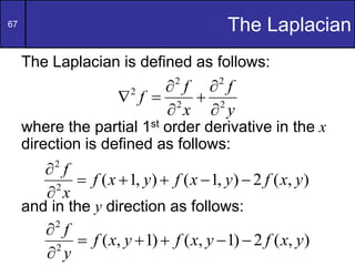
68. 68 The Laplacian (cont…)
So, the Laplacian can be given as follows:
We can easily build a filter based on this
)
,
1
(
)
,
1
(
[
2
y
x
f
y
x
f
f 




)]
1
,
(
)
1
,
( 


 y
x
f
y
x
f
)
,
(
4 y
x
f

0 1 0
1 -4 1
0 1 0

69. 69 The Laplacian (cont…)
Applying the Laplacian to an image we get a
new image that highlights edges and other
discontinuities
Original
Image
Laplacian
Filtered Image
Laplacian
Filtered Image
Scaled for Display

70. 70 But That Is Not Very Enhanced!
The result of a Laplacian filtering
is not an enhanced image
We have to do more work in
order to get our final image
Subtract the Laplacian result
from the original image to
generate our final sharpened
enhanced image
Laplacian
Filtered Image
Scaled for Display
f
y
x
f
y
x
g 2
)
,
(
)
,
( 



71. 71 Laplacian Image Enhancement
In the final sharpened image edges and fine
detail are much more obvious
- =
Original
Image
Laplacian
Filtered Image
Sharpened
Image

72. 72 Laplacian Image Enhancement

73. 73 Simplified Image Enhancement
The entire enhancement can be combined
into a single filtering operation
)
,
1
(
)
,
1
(
[
)
,
( y
x
f
y
x
f
y
x
f 




)
1
,
(
)
1
,
( 


 y
x
f
y
x
f
)]
,
(
4 y
x
f

f
y
x
f
y
x
g 2
)
,
(
)
,
( 


)
,
1
(
)
,
1
(
)
,
(
5 y
x
f
y
x
f
y
x
f 




)
1
,
(
)
1
,
( 


 y
x
f
y
x
f

74. 74 Simplified Image Enhancement (cont…)
This gives us a new filter which does the
whole job for us in one step
0 -1 0
-1 5 -1
0 -1 0

75. 75 Simplified Image Enhancement (cont…)

76. 76 Variants On The Simple Laplacian
There are lots of slightly different versions of
the Laplacian that can be used:
0 1 0
1 -4 1
0 1 0
1 1 1
1 -8 1
1 1 1
-1 -1 -1
-1 9 -1
-1 -1 -1
Simple
Laplacian
Variant of
Laplacian

77. 77 Revisit 1st Derivative
• The derivative of an image results in a
sharpened image.
• Image derivatives can be computed using
the gradient:

78. 78 Gradient
• The gradient is a vector which has
magnitude and direction:

79. 79 Gradient (cont’d)
• Gradient magnitude: provides
information about edge strength.
• Gradient direction: perpendicular to
the direction of the edge (useful for
tracing object boundaries).

80. 80 Gradient Computation
• Approximate partial derivatives using finite
differences:
Δx
232 177 82 7
241 18 152 140
156 221 67 3
100 45 1 103
 
 
 
 
 
 
x
y
Notation:

81. 81 Implement Gradient Using Masks
• We can implement and using
masks:
(x+1/2,y)
(x,y+1/2)
*
*
good approximation
at (x+1/2,y)
good approximation
at (x,y+1/2)
Derivatives are not
computed at the same
location!

82. 82 Implement Gradient Using Masks (cont’d)
• A different approximation of the
gradient:
• We can implement and using the following masks:
*
(x+1/2,y+1/2)
good approximation
Derivatives are
computed at the
same location!

83. 83 Example: Gradient Magnitude Image
Gradient Magnitude
(isotropic, i.e.,
edges in all directions)
• The gradient magnitude can be visualized as an image by mapping
the values to [0, 255]

84. 84 Implement Gradient Using Masks (cont’d)
• Other approximations
Sobel
Prewitt

85. 85 Sobel Example
Sobel filters are typically used for edge
detection
An image of a
contact lens which
is enhanced in
order to make
defects (at four
and five o’clock in
the image) more
obvious

86. 86 Laplacian vs Gradient
Laplacian Sobel
• Laplacian localizes edges better (zero-crossings).
• Higher order derivatives are typically more sensitive to noise.
• Laplacian is less computational expensive (i.e., one mask).
• Laplacian can provide edge magnitude information
but no information about edge direction.

87. 87 1st & 2nd Derivatives
Comparing the 1st and 2nd derivatives we
can conclude the following:
– 1st order derivatives generally produce thicker
edges (if thresholded at ramp edges)
– 2nd order derivatives have a stronger
response to fine detail e.g. thin lines
– 1st order derivatives have stronger response
to grey level step
– 2nd order derivatives produce a double
response at step changes in grey level (which
helps in detecting zero crossings)

88. 88 Unsharp masking
Used by the printing industry
Subtracts an unsharped (smooth) image
from the original image f(x,y).
–Blur the image
b(x,y)=Blur{f(x,y)}
–Subtract the blurred image from the original
(the result is called the mask)
gmask(x,y)=f(x,y)-b(x,y)
–Add the mask to the original
g(x,y)=f(x,y)+k gmask(x,y) with k non negative

89. 89 Unsharp masking (cont...)
Sharping mechanism
When k>1 the process is
referred to as highboost filtering

90. 90 Unsharp masking (cont...)
Original image
Blurred image
Mask
Unsharp masking
Highboost filtering (k=4.5)

91. 91
Combining Spatial Enhancement
Methods
Successful image
enhancement is typically not
achieved using a single
operation
Rather we combine a range
of techniques in order to
achieve a final result
This example will focus on
enhancing the bone scan to
the right

92. 92
Combining Spatial Enhancement
Methods (cont…)
Laplacian filter of
bone scan (a)
Sharpened version of
bone scan achieved
by subtracting (a)
and (b) Sobel filter of bone
scan (a)
(a)
(b)
(c)
(d)

93. 93
Combining Spatial Enhancement
Methods (cont…)
The product of (c)
and (e) which will be
used as a mask
Sharpened image
which is sum of (a)
and (f)
Result of applying a
power-law trans. to
(g)
(e)
(f)
(g)
(h)
Image (d) smoothed with
a 5*5 averaging filter

94. 94
Combining Spatial Enhancement
Methods (cont…)
Compare the original and final images

95. 95 Summary
In this lecture we have looked at the idea of
spatial filtering and in particular:
– Neighbourhood operations
– The filtering process
– Smoothing filters
– Dealing with problems at image edges when
using filtering
– Correlation and convolution
– Sharpening filters
– Combining filtering techniques