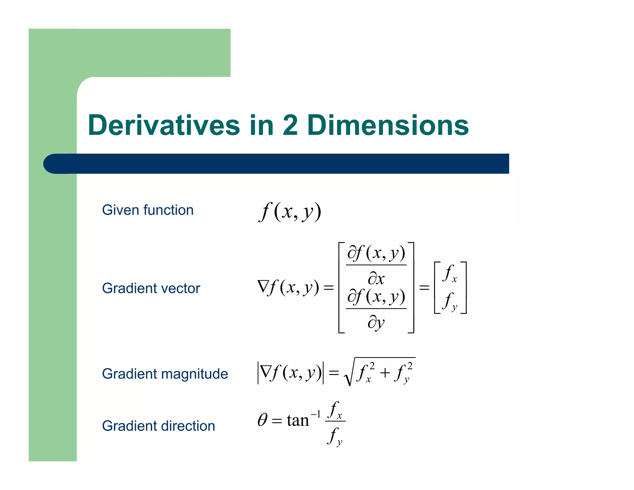
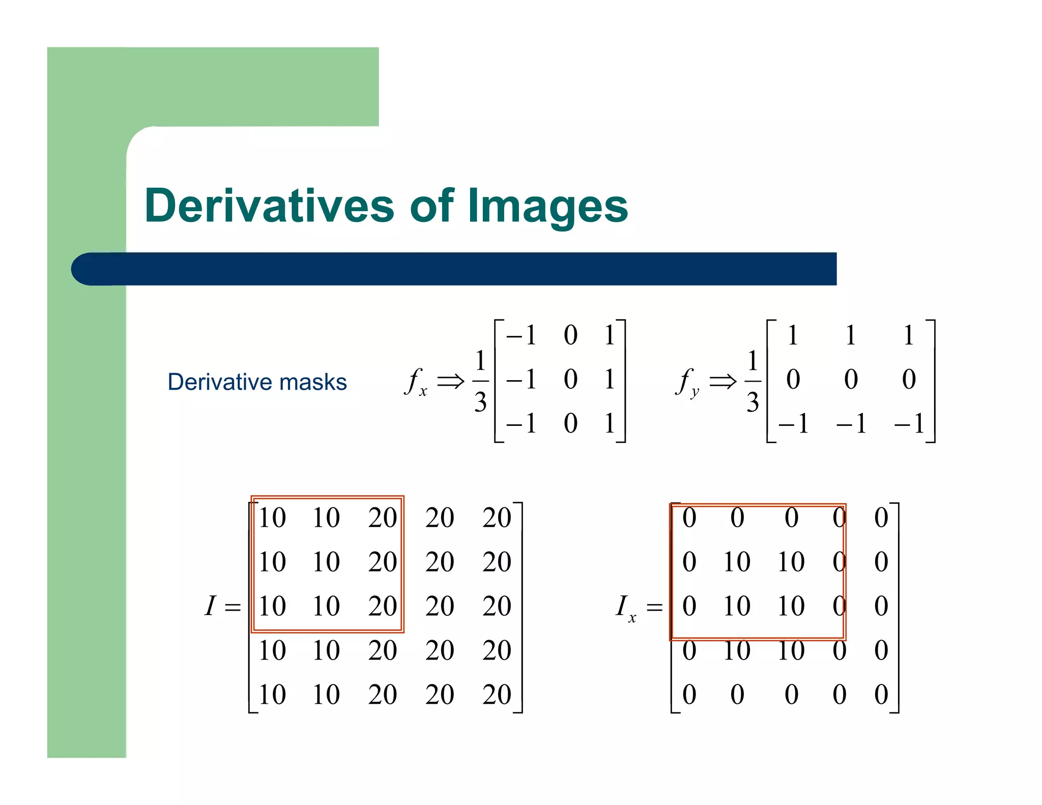
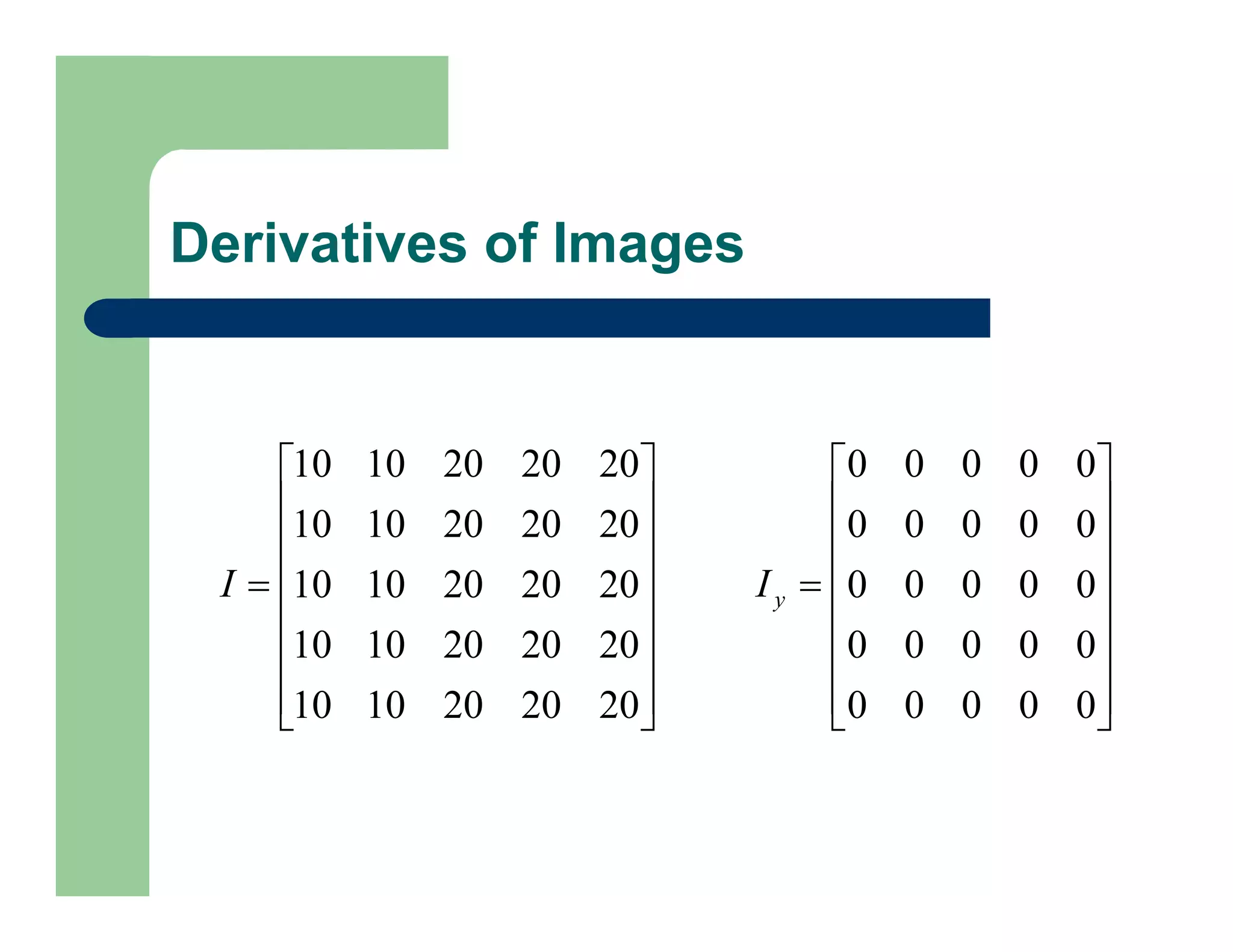
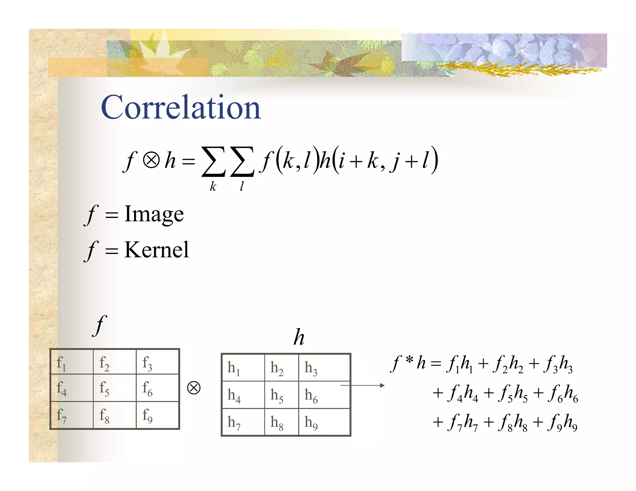
The document outlines concepts in computer vision, specifically focusing on image filtering techniques, image noise, and derivatives. It covers various types of images (binary, grayscale, color), the effect of noise on pixel values, and mathematical definitions of derivatives. Additionally, it provides examples of discrete derivatives, convolution operations, and MATLAB functions for implementing these concepts in image processing.

1. CAP 5415 Computer Vision
Fall 2011
Dr. Mubarak Shah
Univ. of Central Florida
www.cs.ucf.edu/~vision/courses/cap5415/fall2012
Office 247-F HEC

2. Filtering
Lecture-2

3. General
 Binary
 Gray Scale
 Color

4. Binary Images
0: Black
1: White p
q
X
Y
Row 1
Row q
1 1 1
0 0 0 0
0
1

5. Gray Level Image
10 5 9
100

6. Gray Scale Image

7. Color Image
Red, Green, Blue Channels

8. Image Histogram

9. Image Noise
 Light Variations
 Camera Electronics
 Surface Reflectance
 Lens

10. Image Noise
 I(x,y) : the true pixel values
 n(x,y) : the noise at pixel (x,y)
     
y
x
n
y
x
I
y
x
I ,
,
,
ˆ 



11. Gaussian Noise
  2
2
2
, 
n
e
y
x
n



12. Image Derivatives & Averages

13. Definitions
 Derivative: Rate of change
– Speed is a rate of change of a distance
– Acceleration is a rate of change of speed
 Average (Mean)
– Dividing the sum of N values by N

14. Derivative
x
x f
x
f
x
x
x
f
x
f
dx
df







 
 )
(
)
(
)
(
lim 0
on
accelerati
speed
dt
dv
a
dt
ds
v 


15. Examples
3
4
2
4
2 x
x
dx
dy
x
x
y




x
x
e
x
dx
dy
e
x
y







)
1
(
cos
sin

16. Discrete Derivative
)
(
)
(
)
(
lim 0 x
f
x
x
x
f
x
f
dx
df
x






 

)
(
1
)
1
(
)
(
x
f
x
f
x
f
dx
df





)
(
)
1
(
)
( x
f
x
f
x
f
dx
df






17. Discrete Derivative
Finite Difference
)
(
)
1
(
)
1
( x
f
x
f
x
f
dx
df






)
(
)
1
(
)
( x
f
x
f
x
f
dx
df





)
(
)
1
(
)
( x
f
x
f
x
f
dx
df




 Backward difference
Forward difference
Central difference

18. Example
0
5
20
15
5
10
5
0
)
(
0
0
5
15
0
5
5
0
)
(
20
20
20
25
10
10
15
10
)
(









x
f
x
f
x
f
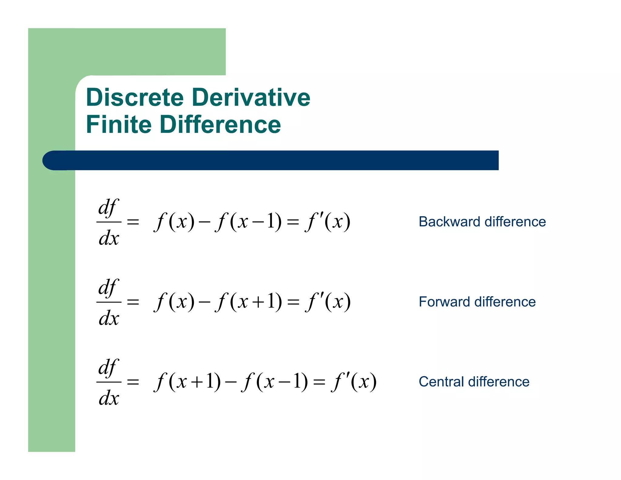
Derivative Masks
Backward difference
Forward difference
Central difference
[-1 1]
[1 -1]
[-1 0 1]

19. Derivatives in 2 Dimensions
)
,
( y
x
f
Given function

























y
x
f
f
y
y
x
f
x
y
x
f
y
x
f )
,
(
)
,
(
)
,
(
Gradient vector
2
2
)
,
( y
x f
f
y
x
f 


Gradient magnitude
y
x
f
f
1
tan


Gradient direction

20. Derivatives of Images














1
0
1
1
0
1
1
0
1
3
1
x
f
Derivative masks














1
1
1
0
0
0
1
1
1
3
1
y
f

















20
20
20
10
10
20
20
20
10
10
20
20
20
10
10
20
20
20
10
10
20
20
20
10
10
I

















0
0
0
0
0
0
0
10
10
0
0
0
10
10
0
0
0
10
10
0
0
0
0
0
0
x
I

21. Derivatives of Images

















0
0
0
0
0
0
0
0
0
0
0
0
0
0
0
0
0
0
0
0
0
0
0
0
0
y
I

















20
20
20
10
10
20
20
20
10
10
20
20
20
10
10
20
20
20
10
10
20
20
20
10
10
I

22. Correlation
   
 



k l
l
j
k
i
h
l
k
f
h
f ,
,
Kernel
Image


f
f
h1 h2 h3
h4 h5 h6
h7 h8 h9
h
f1 f2 f3
f4 f5 f6
f7 f8 f9

9
9
8
8
7
7
6
6
5
5
4
4
3
3
2
2
1
1
*
h
f
h
f
h
f
h
f
h
f
h
f
h
f
h
f
h
f
h
f









f

23. Convolution
   
 


k l
l
j
k
i
h
l
k
f
h
f ,
,
*
Kernel
Image


h
f h7 h8 h9
h4 h5 h6
h1 h2 h3
h9 h8 h7
h6 h5 h4
h3 h2 h1
h1 h2 h3
h4 h5 h6
h7 h8 h9
h
flip
X 
flip
Y 
f1 f2 f3
f4 f5 f6
f7 f8 f9

1
9
2
8
3
7
4
6
5
5
6
4
7
3
8
2
9
1
*
h
f
h
f
h
f
h
f
h
f
h
f
h
f
h
f
h
f
h
f









f

24. Convolution
x
x
f
h
)
1
,
1
(
)
1
,
1
(
)
1
,
0
(
)
1
,
(
)
1
,
1
(
)
1
,
1
(
)
0
,
1
(
)
,
1
(
)
0
,
0
(
)
,
(
)
0
,
1
(
)
,
1
(
)
1
,
1
(
)
1
,
1
(
)
1
,
0
(
)
1
,
(
)
1
,
1
(
)
1
,
1
(
)
,
(
h
y
x
f
h
y
x
f
h
y
x
f
h
y
x
f
h
y
x
f
h
y
x
f
h
y
x
f
h
y
x
f
h
y
x
f
h
y
x
f





























 





1
1
1
1
)
,
(
)
,
(
i j
j
i
h
i
y
i
x
f
h
f
-1,0 0,1 1,1
-1,0 0,0 1,0
-1,-1 0,-1 1,-1
Coordinates

25. Averages
 Mean
n
I
n
I
I
I
I
n
i
i
n





 1
2
1 
 Weighted mean
n
I
w
n
I
w
I
w
I
w
I
n
i
i
i
n
n






 1
2
2
1
1 

26. Gaussian Filter
2
2
2
)
( 
x
e
x
g


 
011
.
13
.
6
.
1
6
.
13
.
011
.
)
( 
x
g
2
2
2
2
(
)
,
( 
y
x
e
y
x
g



1



27. Properties of Gaussian
 Most common natural model
 Smooth function, it has infinite number of
derivatives
 Fourier Transform of Gaussian is Gaussian.
 Convolution of a Gaussian with itself is a
Gaussian.
 There are cells in eye that perform Gaussian
filtering.

28. Alper Yilmaz, Mubarak Shah, UCF
Filtering
 Modify pixels based on some function of the
neighborhood
10 30 10
20 11 20
11 9 1
5.7
 
p
f

29. Linear Filtering
 The output is the linear combination of the
neighborhood pixels
1 3 0
2 10 2
4 1 1
Image
1 0 -1
1 0.1 -1
1 0 -1
Kernel
= 5
Filter Output

Alper Yilmaz, Mubarak Shah, UCF

30. Filtering Examples
0 0 0
0 1 0
0 0 0
* 
Alper Yilmaz, Mubarak Shah, UCF

31. Filtering Examples
0 0 0
0 0 1
0 0 0
* 
Alper Yilmaz, Mubarak Shah, UCF

32. Filtering Examples
1 1 1
1 1 1
1 1 1
9
1
* 
Alper Yilmaz, Mubarak Shah, UCF

33. Filtering Examples
1 1 1 1 1
1 1 1 1 1
1 1 1 1 1
1 1 1 1 1
1 1 1 1 1
25
1
* 
Alper Yilmaz, Mubarak Shah, UCF

34. Blurring Examples
original
original
pixel offset
pixel offset
filtered
filtered
0
0
8
8
4
0.3
0.3
2.4
8
4
6
4.8

35. Filtering Gaussian
* 
Alper Yilmaz, Mubarak Shah, UCF

36. Gaussian vs. Smoothing
Gaussian Smoothing Smoothing by Averaging
Alper Yilmaz, Mubarak Shah, UCF

37. Noise Filtering
Gaussian Noise
After Gaussian Smoothing
After Averaging
Alper Yilmaz, Mubarak Shah, UCF

38. MATLAB Functions
 conv: 1-D Convolution.
– C = conv(A, B) convolves vectors A and B.
 conv2: Two dimensional convolution.
– C = conv2(A, B) performs the 2-D convolution
of matrices A and B.

39. MATLAB Functions
 filter2: Two-dimensional digital filter.
– Y = filter2(B,X) filters the data in X with the 2-D
FIR filter in the matrix B.
– The result, Y, is computed using 2-D correlation and is
the same size as X.
– filter2 uses CONV2 to do most of the work. 2-
D correlation is related to 2-D convolution by a
180 degree rotation of the filter matrix.

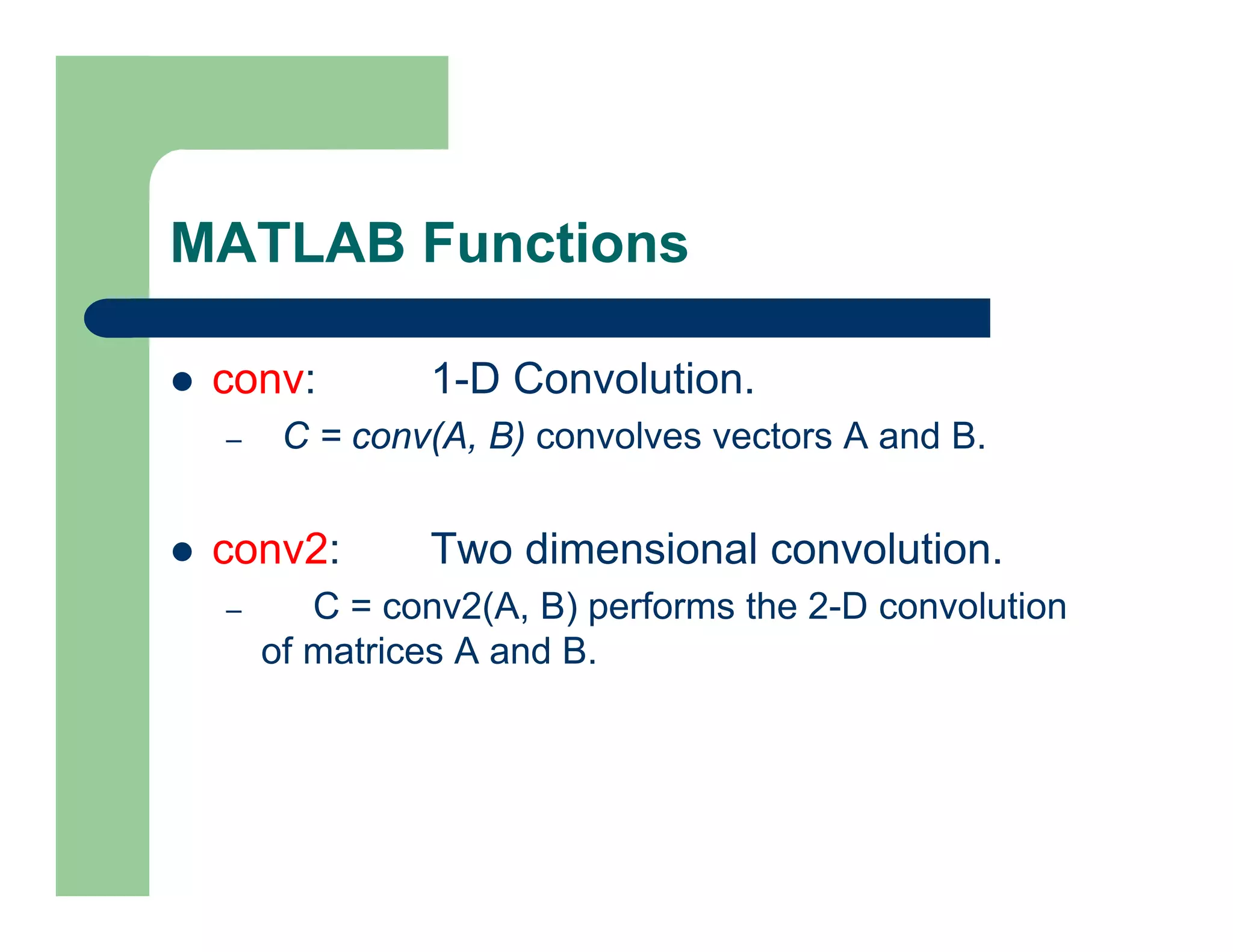
40. MATLAB Functions
 gradient: Approximate gradient.
– [FX,FY] = gradient(F) returns the numerical
gradient of the matrix F. FX corresponds to dF/dx,
FY corresponds to dF/dy.
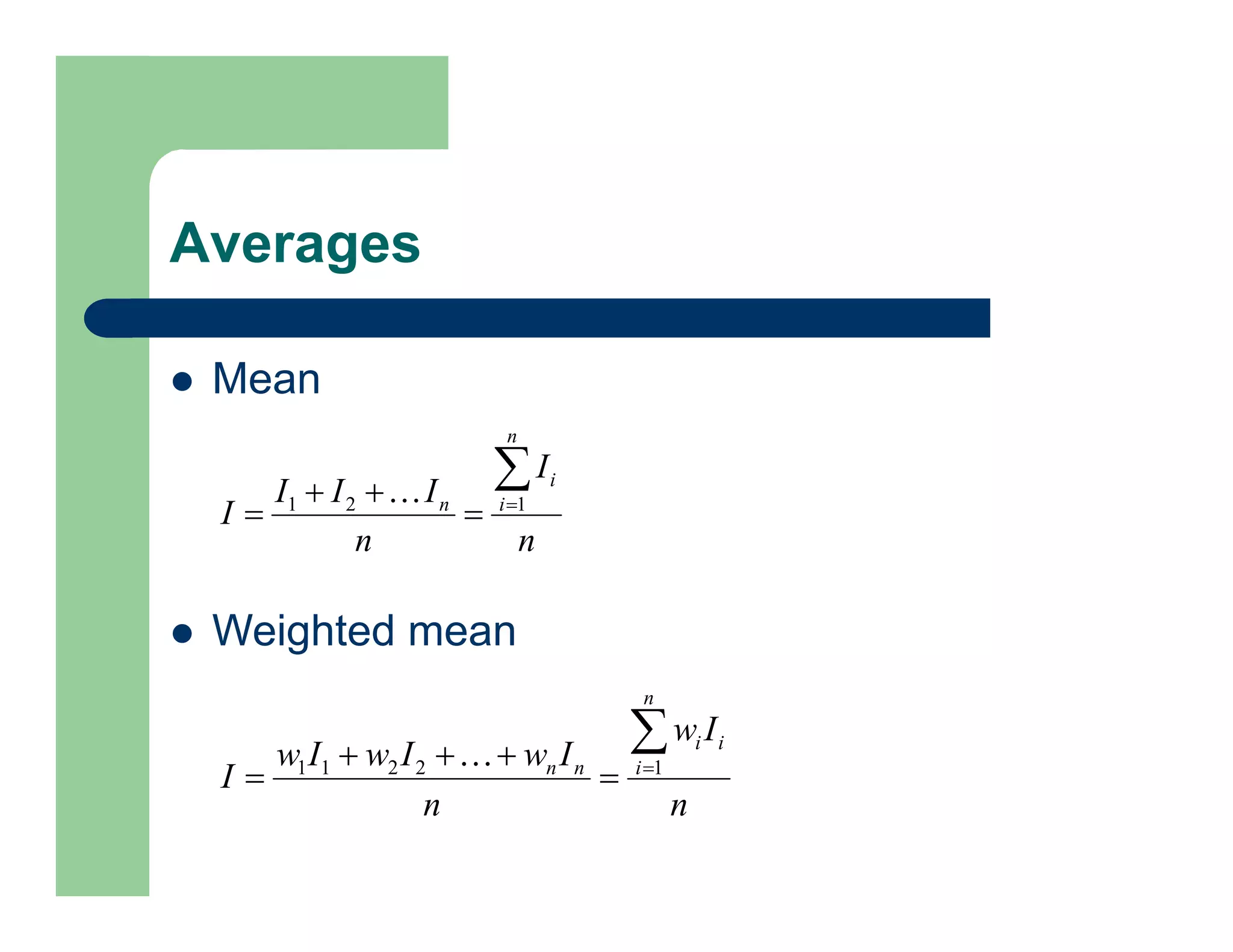
 mean: Average or mean value.
– For vectors, mean(X) is the mean value
(average) of the elements in X.

41. MATLAB Functions
 special: Create predefined 2-D filters
– H = fspecial(TYPE) creates a two-dimensional filter H of the
specified type. Possible values for TYPE are:
– 'average' averaging filter;
– 'gaussian' Gaussian lowpass filter
– 'laplacian' filter approximating the 2-D Laplacian operator
– 'log' Laplacian of Gaussian filter
– 'prewitt' Prewitt horizontal edge-emphasizing filter
– 'sobel' Sobel horizontal edge-emphasizing filter
– Example: H=fspecial('gaussian',7,1) creates a 7x7 Gaussian
filter with variance 1.