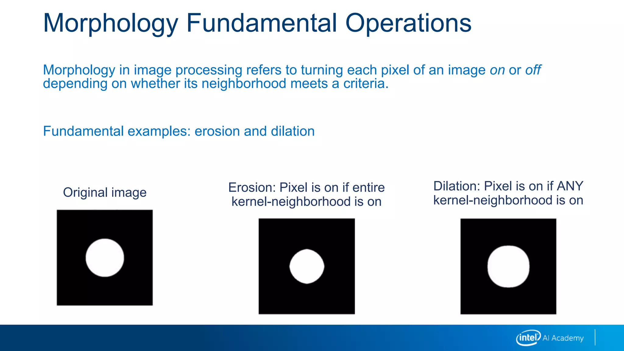
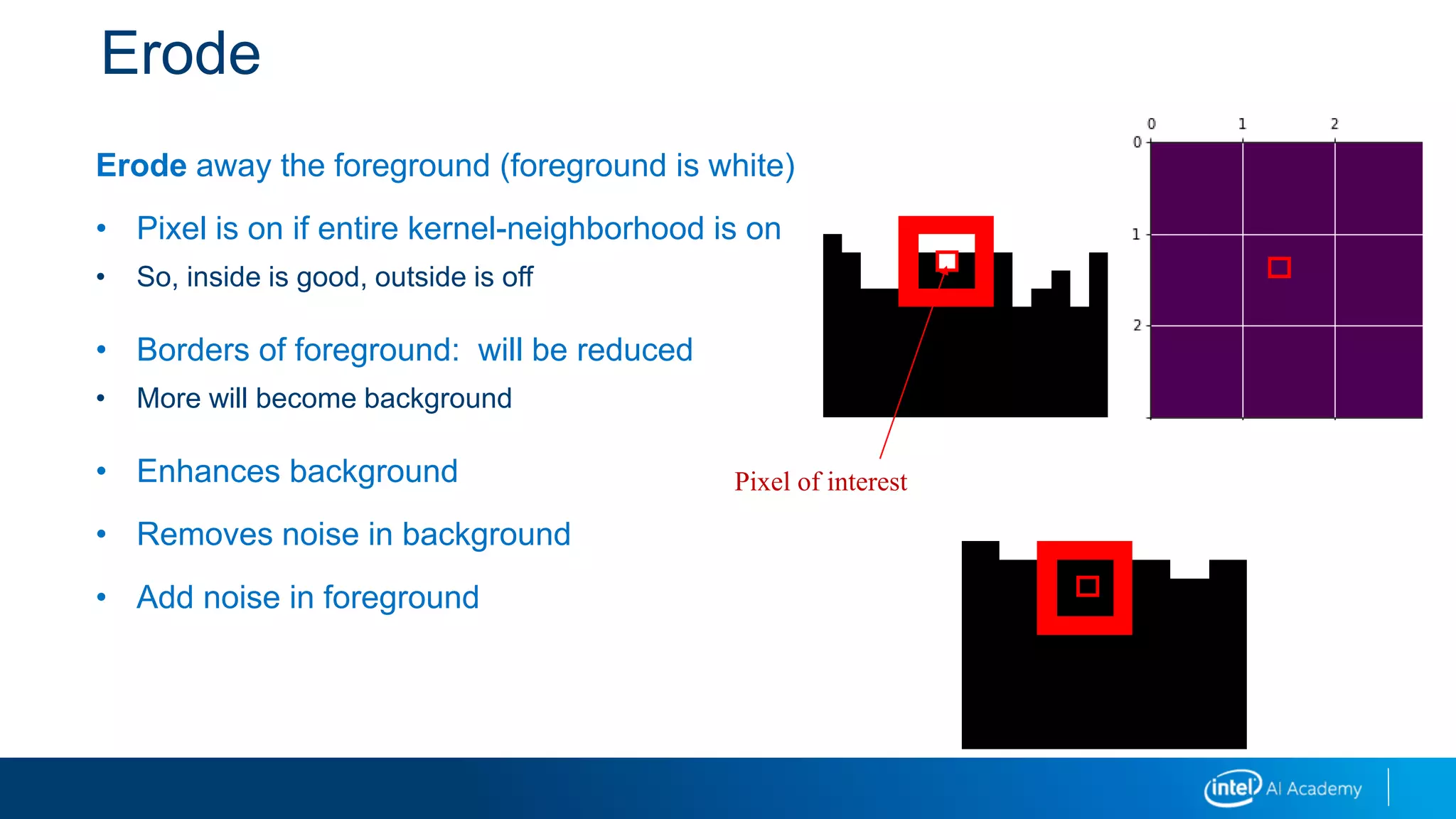
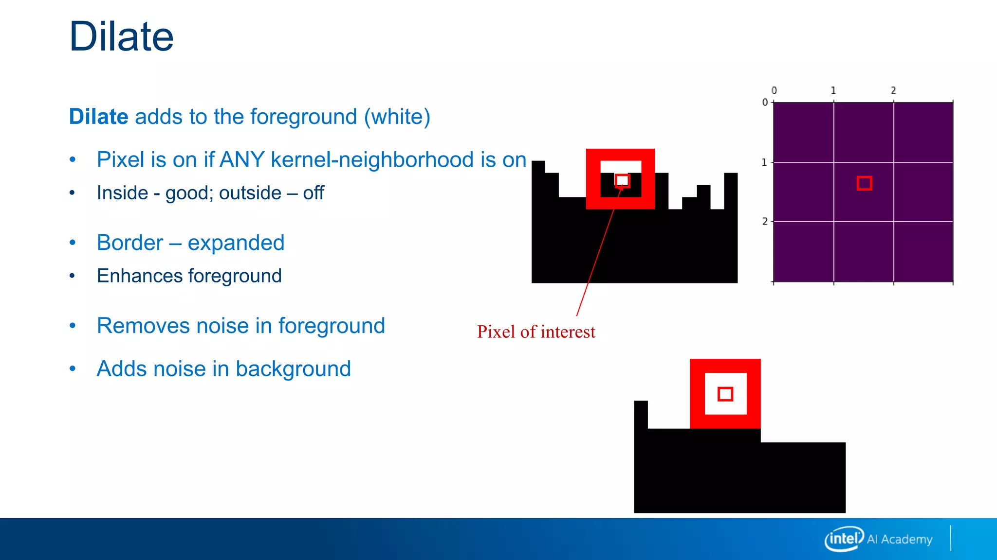
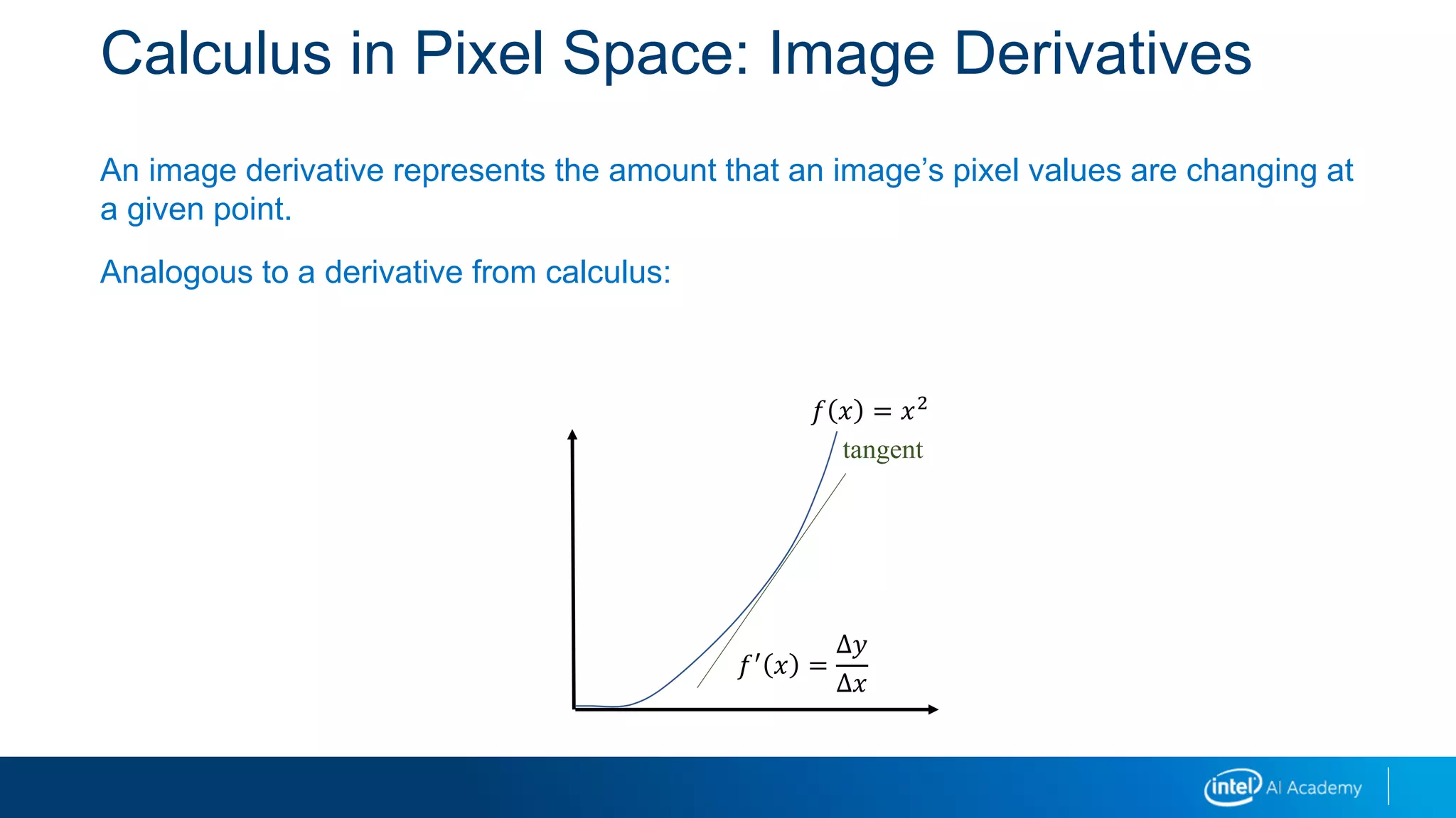
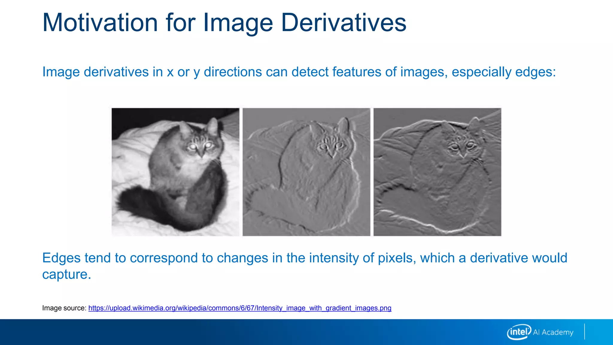
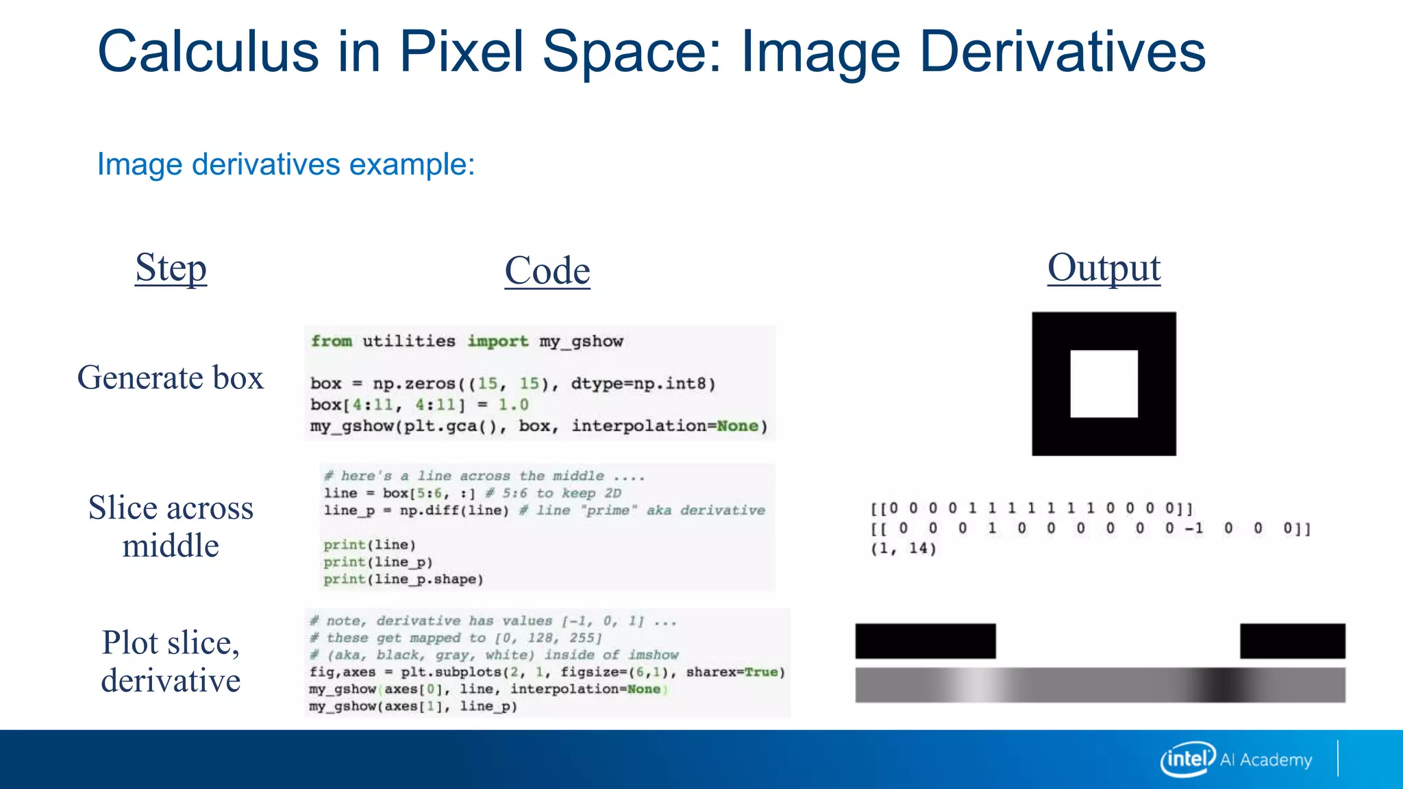
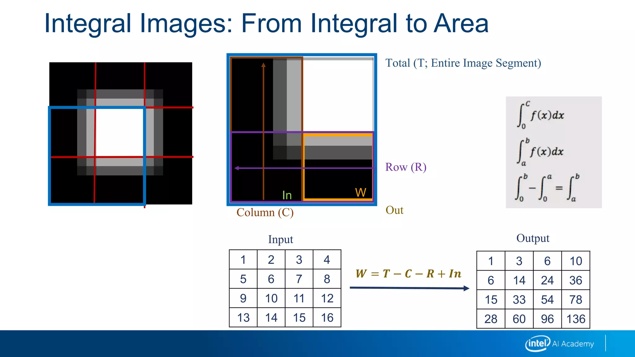
The document discusses image processing techniques including image derivatives, integral images, convolution, morphology operations, and image pyramids. It explains that image derivatives detect edges by capturing changes in pixel intensity, and provides an example calculation. Integral images allow fast computation of box filters by precomputing pixel sums. Convolution is used to calculate probabilities as the sliding overlap of distributions. Morphology operations like erosion and dilation modify images based on pixel neighborhoods. Image pyramids create multiple resolution layers that aid in object detection across scales.

1. Part I

2. Legal Notices and Disclaimers
This presentation is for informational purposes only. INTEL MAKES NO WARRANTIES,
EXPRESS OR IMPLIED, IN THIS SUMMARY.
Intel technologies’ features and benefits depend on system configuration and may require
enabled hardware, software or service activation. Performance varies depending on system
configuration. Check with your system manufacturer or retailer or learn more at intel.com.
This sample source code is released under the Intel Sample Source Code License
Agreement.
Intel and the Intel logo are trademarks of Intel Corporation in the U.S. and/or other countries.
*Other names and brands may be claimed as the property of others.
Copyright © 2018, Intel Corporation. All rights reserved.
2

3. Calculus in Pixel Space: Image Derivatives
An image derivative represents the amount that an image’s pixel values are changing at
a given point.
Analogous to a derivative from calculus:
tangent
𝑓′
𝑥 =
Δ𝑦
Δ𝑥
𝑓 𝑥 = 𝑥2

4. Motivation for Image Derivatives
Image derivatives in x or y directions can detect features of images, especially edges:
Edges tend to correspond to changes in the intensity of pixels, which a derivative would
capture.
Image source: https://upload.wikimedia.org/wikipedia/commons/6/67/Intensity_image_with_gradient_images.png

5. Calculus in Pixel Space: Image Derivatives
Image derivatives example:
Step
Generate box
Slice across
middle
Plot slice,
derivative
Code Output

6. Integral Images
Many applications
Fast calculation of Haar wavelets in face recognition
Precomputing can speed up application of multiple box filters
Can be used to approximate other (non-box) kernels
Method
Summed area table is precalculated
 Pixel values from origin
 Recursive algorithm used
y = f(x)
Area = ⎰ f(x).dx
a
b
a b

7. Integral Images: From Integral to Area
Out
WIn
Column (C)
Row (R)
Total (T; Entire Image Segment)
𝑾 = 𝑻 − 𝑪 − 𝑹 + 𝑰𝒏
1 2 3 4
5 6 7 8
9 10 11 12
13 14 15 16
Input
1 3 6 10
6 14 24 36
15 33 54 78
28 60 96 136
Output

9. Dice Probability
Probability of a 2 .... given by:
1. Taking all combinations of events.
2. Computing sums.
3. Returning counts of 2 events divided by total number of events.
4. Also, we know this is 1/6 * 1/6
die = np.full(6, 1/6.0)print(die)
np.convolve(die, die, mode='full')

10. Dice Probability: Convolution
Probability of a each outcome…
0.0278
0.0556
0.0833
0.111
0.1389
0.1667
0.1389
0.1111
0.0833
0.0556
0.0278
Box graphic from: https://commons.wikimedia.org/wiki/Category:Dice_probability#/media/File:Twodice.svg
Dice graphic from: https://commons.wikimedia.org/wiki/Category:6-sided_dice#/media/File:6sided_dice.jpg

11. Probability as a Sliding Window
In the dice example, to get, say, a total
of 7:
• We can fix a point 7 and slide the two arrays past
(one in reverse order).
• And when they add up to seven, we take that
sum-product.
1 2 3 4 5 6
6 5 4 3 2 1
1 2 3 4 5 6
6 5 4 3 2 1
1 2 3 4 5 6
6 5 4 3 2 1
1 2 3 4 5 6
6 5 4 3 2 1
Ways to get 12
Ways to get 10
Ways to get 8
Ways to get 7P(s=2) = P1( )* P2( )
P(s=3) = P1( )* P2( ) + P1( )* P2( )
𝑃 𝑠 = 𝑇 =
𝑖
𝑃(𝑖)𝑃(𝑇 − 𝑖)
𝑃 𝑇 =
𝑖+𝑗=𝑇
𝑃 𝑖 𝑃(𝑗)

12. Probability as a Convolution
In general, the probability of sums of events is the convolution of the probabilities of the
component events.
In general, in mathematics, a convolution is a function h produced by a function g
“operating” on another function f. This is usually written:
Here, the distribution of probabilities for two dice (h) is a convolution of the probability
distribution over the first die (f) with the probability distribution over the second die (g).
𝑓⨂𝑔 = ℎ

13. Probability as a Convolution
Dice probability is a convolution:
Sum over all the right rolls (r) so that the events add up to our desired total T
Note: r + (T - r) = T
Could also write it like this: And in general like this:
Those sums are convolutions!
Here, we've convolved a discrete function with itself.
Just like we'll do with images, except images are 2D.
𝑃 2 = 𝑃 1 ∗ 𝑃(1)
𝑃 3 =
𝑟=1,2
𝑃 𝑟 ∗ 𝑃 𝑇 − 𝑟 = 𝑃 1 ∗ 𝑝 2 + 𝑃 2 ∗ 𝑃(1)

14. Probability as a Convolution
Dice example with code:
Step Code & Output
Generate dice probability
distribution
Convolve to get overall
probabilities

15. A General 2D Convolution
The usual formula looks like this:
But, as an idea, that is less than clear!
𝑓 ⊗ 𝑔 𝑁, 𝑀 =
”𝑟𝑖𝑔ℎ𝑡”𝑖𝑗,𝑘𝑙
𝑓 𝑖, 𝑘 𝑔[𝑗, 𝑙]𝑓 ⊗ 𝑔 𝑁 =
𝑜𝑓𝑓𝑠𝑒𝑡𝑠
𝑓 𝑜𝑓𝑓𝑠𝑒𝑡 𝑔[𝑁 − 𝑜𝑓𝑓𝑠𝑒𝑡]
𝑖𝑚𝑔 ⊗ 𝑘𝑒𝑟𝑛 𝑅, 𝐶 =
𝑝𝑖𝑥𝑒𝑙_𝑝𝑎𝑖𝑟
𝑖𝑛𝑎𝑙𝑖𝑔𝑛𝑒𝑑
𝑛𝑒𝑖𝑔ℎ𝑏𝑜𝑟ℎ𝑜𝑜𝑑𝑠
(𝑘𝑒𝑟𝑛,𝑅,𝐶)
𝑖𝑚𝑔 𝑖𝑚𝑔𝑟, 𝑖𝑚𝑔𝑐 𝑘𝑒𝑟𝑛[𝑘𝑒𝑟𝑛𝑟, 𝑘𝑒𝑟𝑛𝑐]
result
imgr, imgc
kernr, kernc
given a kernel, and R, C…
this tells us the corresponding
pixels in img and elements in
kernel
a pixel

16. 2D Convolution
A combination of a sliding window as it moves over a 2D image
We align the kernel with a block of the image at an anchor point
In the probability example, our anchor point was a Total
The resulting value at the anchor point is the dot-product of the aligned regions
Dot-product means multiply elements pairwise and then sum

17. 2D Convolution
The probability formula and the 2D convolution formula have these pieces:
Multiply element wise
Sum the products
Align
The alignment determines the values we sum over and the values passed to the
functions inside the sum:
Total anchored the probabilities
For a 2D convolution, a target pixel at R,C anchors the neighborhoods of the image and
the kernel

18. Manual 2D Convolution with SciPy
convolve2d(box, kernel, mode)
With mode=‘same’ or mode=‘full’ we have to pad
§ Can use wrapping
§ Symmetric
§ Fill value

20. Kernel Methods
Kernel methods involve taking a convolution of a kernel - a small array -
with an image to detect the presence of features at locations on an
image.
Also called filtering methods.
Images are filtered using neighborhood operators.
Separable filtering:
2D can be applied as sequential 1D (first a horizontal filter, then a vertical filter).

21. Low-Pass Filters
Linear methods:
• Box (mean)
• Gaussian blur (weighted sum)
Non-linear methods:
• Bilateral filter (combination of a Gaussian and a empirical similarity of the
neighborhood to the center pixel)
• Median blur

22. Blurring

23. Blurring and Smoothing Using Bilateral Filter
Bilateral smooths both intensities and colors
Edge preserving will produce a watercolor effect when repeated
Pixel distance -and- "color distance"

24. Kernel Application Details
Padding – border effects
Constant
Replicate the edge pixel value
Wrap around to other side of image
Mirror back toward center of image

26. Erosion: Pixel is on if entire
kernel-neighborhood is on
Morphology Fundamental Operations
Morphology in image processing refers to turning each pixel of an image on or off
depending on whether its neighborhood meets a criteria.
Fundamental examples: erosion and dilation
Dilation: Pixel is on if ANY
kernel-neighborhood is on
Original image

27. Morphology Fundamental Operations
Binary image operations: formal definitions
Morphological operations
Dilation dilate(f,s) = c > 1
on if any in neighborhood are on
Erosion erode(f,s) = c = S
on if all in neighborhood are on
Majority maj(f,s) = c > S/2
on if most in neighborhood are on
s= structuring element f = binary image
S= size of structuring element
c = count in aligned neighborhood after multiplying f and s

28. Erode
Erode away the foreground (foreground is white)
• Pixel is on if entire kernel-neighborhood is on
• So, inside is good, outside is off
• Borders of foreground: will be reduced
• More will become background
• Enhances background
• Removes noise in background
• Add noise in foreground
Pixel of interest

29. Dilate
Dilate adds to the foreground (white)
• Pixel is on if ANY kernel-neighborhood is on
• Inside - good; outside – off
• Border – expanded
• Enhances foreground
• Removes noise in foreground
• Adds noise in background
Pixel of interest

30. Morphology: Additional Operations
Binary image operations
Morphological operations
Opening open(f,s) = dilate(erode(f,s), s)
Closing close(f,s) = erode(dilate(f,s), s)
s= structuring element
f = binary image
S= size of structuring element
c = count

31. Other Relationships: Open
Opening: dilate(erode(img))
• Erode it, then dilate it
• Remove outside noise (false foreground); remove local peaks
• Count objects
• opening = cv2.morphologyEx(img, cv2.MORPH_OPEN, kernel)

32. Other Relationships: Close
Closing: erode(dilate(img))
• Remove inside noise (false background)
• Used as a step in connected-components analysis
closing = cv2.morphologyEx(img, cv2.MORPH_CLOSE, kernel)
Iterations of these are erode(erode(dilate(dilate())))
 ei(di(img))
gradient = dilation - erosion
 finds boundary
gradient = cv2.morphologyEx(img, cv2.MORPH_GRADIENT, kernel

33. Other Relationships: Tophat/Blackhat
Isolate brighter/dimmer (tophat/blackhat) than their surroundings
Tophat: image – opening
tophat = cv2.morphologyEx(img, cv2.MORPH_TOPHAT, kernel)
Blackhat: closing – image
blackhat = cv2.morphologyEx(img, cv2.MORPH_BLACKHAT, kernel)
These can be related to other mathematical techniques:
• Max-pool in neural network layers is a dilation using a square structuring element followed by
downsample (1/p).
• It is possible to learn the operations; for example, as implicit layers in the neural network.

35. Image Pyramids
A stack of images at different resolutions is an image pyramid.
• Use when you are unsure of object sizes in an image
Work with images of different resolutions and find object in each
• Uses Gaussian and Laplacian layers

36. Gaussian Pyramid
Having multiple resolutions represented
simultaneously.
Working with lower-resolution images allows for
faster computations.
Each Gaussian level loses information:
• Create a complementary Laplacian Pyramid, which
holds that information
• Bottom Gaussian level plus all Laplacian levels
reconstructs the original image

37. Pyramids
Gaussian Pyramid Laplacian Pyramid

38. Example Laplacian Level
𝐿𝑜 = 𝐺𝑜 − 𝑈𝑃 𝐺1 ⊗ Gaus5x5 = 𝐺𝑜 − 𝑃𝑦𝑟𝑈𝑝 𝐺1

39. Laplacian Pyramid (pyrUp/pyrDown)
Power of 2 for biggest image sizes
• This makes halving/doubling work well
• Can also pad out to next power of 2
Expanding:
𝑔0 = 𝑙0 + 𝑈𝑃 𝑔1 = 𝑙0 + 𝑈𝑃 𝑙1 + 𝑈𝑃 𝑔2 = 𝑙0 + 𝑈𝑃(𝑙1 + 𝑈𝑃 𝑏𝑎𝑠𝑒 )

40. Using Image Pyramids for Blending
Combining two images seamlessly (image
stitching and compositions)
1. Decompose source images into Laplacian
pyramid.
2. Create a Gaussian mask from the binary
mask image.
3. Compute the sum of the two weighted
pyramids to stitch the images together.

42. Edge Detectors
Finding stable features for matching
Matching human boundary detection
Sobel, Scharr, and Laplacian filters

43. Sobel
Most common differentiation operator
Approximates a derivative on discrete grid
• Actually a fit to polynomial
Used for kernels of any size
• Larger kernels are less sensitive to noise, and therefore more accurate
Combine Gaussian smoothing with differentiation
Higher order also (first, second, third, or mixed derivatives)
-1 0 1
-2 0 2
-1 0 1
1 2 1
0 0 0
-1 -2 -1
Sobel x
Sobel y

44. Scharr
Scharr is a specific Sobel case used for computing 3x3
• As fast as Sobel, but more accurate for small kernel sizes
Especially useful when implementing common shape
classifiers
• Need to collect shape information through histograms of gradient
angles
First x- or y- image derivative
• Scharr(src, dst, ddepth, dx, dy, scale, delta, borderType)
• Sobel(src, dst, ddepth, dx, dy, cv_scharr, scale, delta, borderType)
-3 0 3
-10 0 10
-3 0 3
3 10 3
0 0 0
-3 10 3
Scharr x
Scharr y

45. Laplacian
Laplacian function
Can be used to detect edges
Can use 8-bit or 32-bit source image
Often used for blob detection
Local peak and trough in an image will maximize and minimize Laplacian
Sum of second derivatives in x,y
• Works like a second-order Sobel derivative
𝐿𝑎𝑝𝑙𝑎𝑐𝑒 𝑓 =
𝛿2𝑓
𝛿𝑥2
+
𝛿2𝑓
𝛿𝑦2

46. Multiple Colors
Should you detect edges in color or grayscale?
• Typically we do edge detection in grayscale.
• If we want to do edge detection in color…
• If you take the union of edges, you might thicken the edges
• If you take the sum of gradients, you need to be careful about sign cancelation
• Consider non-RGB color space

47. Distance Transform
Once we have edges, we may need to find and group together pixels as an object.
One step in that process is to find the distances from a pixel to a boundary:
1. Invert an edge detector (non-edge is white)
2. Find distance from central points (now white) to nearest edge (now black)