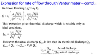
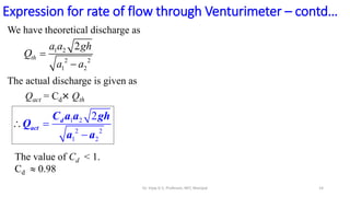
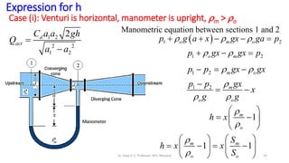
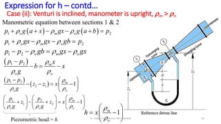
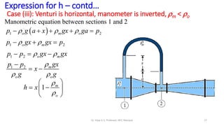
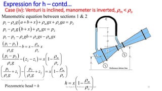
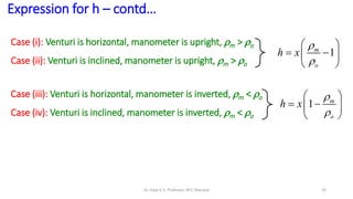
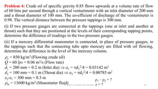
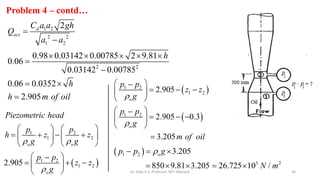
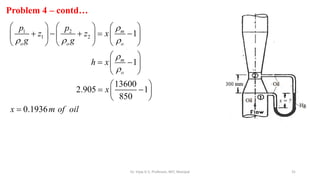
Flow measurement
Flow measurement devices
(An application of the Bernoulli’s equation & Continuity
equation)
Dr. Vijay G. S.
Professor
Dept. of Mech. & Ind. Engg.
MIT, Manipal
email: vijay.gs@manipal.edu
Mob.: 9980032104
Why flow measurement?
In many applications it is required to measure the velocity of flow V or the rate
of flow (discharge) Q through a pipe or an open channel.
• e.g., in a pipe flow it is necessary to know the nature of flow (laminar or
turbulent). By knowing the velocity, one can tell about the nature of flow.
• Or in industrial applications, (say, in a petroleum refinery) it is necessary to
estimate the quantity of fuel produced in a day or a week or a month. This
calls for the measurement of discharge of the fuel through pipes.
• In case of open channels, it is necessary to estimate the distribution of water
to a region of interest. This can be achieved by measuring the discharge of
water through the channel.
2
Dr. Vijay G S, Professor, MIT, Manipal
Flow measuring devices
• There are various methods of flow measurement
• Only some simple and commonly used techniques based on the principles of
fluid mechanics are discussed.
 Bernoulli’s equation
 Continuity equation
3
Dr. Vijay G S, Professor, MIT, Manipal
Flow measurement through pipes:
• An effective way to measure the flowrate through a pipe is to place some type
of restriction or obstruction within the pipe and to measure the pressure
difference between,
(i) the low-velocity, high-pressure upstream section
(ii) the high-velocity, low-pressure downstream section
• The rate of flow of fluid through a pipe is measured by different restriction
devices namely,
 Venturimeter
 Orifice meter
 Pitot tube
 Nozzle meter or flow nozzle
Flow measuring devices – contd…
Restriction
Upstream Downstream
Flow
Low V, High p High V, Low p
4
Dr. Vijay G S, Professor, MIT, Manipal
Venturimeter
Orifice meter
Pitot tube 5
Flow measuring devices – contd…
Dr. Vijay G S, Professor, MIT, Manipal
Flow measurement through open channels:
• Through an open channel the rate of flow is measured by
 Notches
 Weirs
Flow measuring devices – contd…
Rectangular
weir/notch
Triangular
weir/notch Trapezoidal
weir/notch
Notch has a small size and
the weir is a bigger one
6
Dr. Vijay G S, Professor, MIT, Manipal
Venturi Effect:
• The Venturi effect is the reduction in fluid pressure that results when a fluid
flows through a constricted section of pipe.
• The Venturi effect is named after Giovanni Battista Venturi (1746–1822), an
Italian physicist.
Venturimeter
• Fluid flows through a length of
pipe of varying diameter.
• The pressure at “1” is higher than
at “2” because the fluid speed at
“1” is lower than at “2”.
7
Dr. Vijay G S, Professor, MIT, Manipal
Venturimeter – contd…
• A venturimeter or (simply
referred as venturi) is a device
used for measuring the flow rate
of fluid through a pipe.
• It consists of 3 parts:
(i) A short converging part
(ii) Throat
(iii) Diverging part.
• It works on Bernoulli’s
principle.
8
Dr. Vijay G S, Professor, MIT, Manipal
• It is the most precise and most expensive of the three obstruction-type flow
meters.
• The geometry of the Venturimeter is designed to reduce head losses to a
minimum.
Venturimeter – contd…
9
 This is accomplished by
providing a relatively
streamlined contraction and
a very gradual expansion
downstream of the throat
(which eliminates
separation in this
decelerating portion of the
device). Dr. Vijay G S, Professor, MIT, Manipal
10
Venturimeter – contd…
 Most of the head loss that occurs in a well-designed Venturimeter is
due to friction losses along the walls rather than losses associated
with separated flows and the inefficient mixing motion that
accompanies such flow.
• To avoid undue drag, a
Venturimeter typically has an
entry cone of 21 to 30 degrees
and an exit cone of 5 to 15
degrees.
Dr. Vijay G S, Professor, MIT, Manipal
Applying Bernoulli’s equation at
sections 1 and 2 we get,
2 2
1 1 2 2
1 2
2 2
 
    
o o
p V p V
z z
g g g g
As pipe is horizontal, z1 = z2
2 2
1 1 2 2
2 2
 
  
o o
p V p V
g g g g
2 2
1 2 2 1
2 2
 
   
  
   
 
 
o o
p p V V
g g g g
 
1 2


 
o
p p
h
g
But, is the difference of pressure head
at sections 1 and 2
 
1 2


o
p p
g
2 2
2 1
2 2
 
V V
h
g g
Expression for rate of flow through Venturimeter
p2, V2, d2, a2
p1, V1, d1, a1
11
Dr. Vijay G S, Professor, MIT, Manipal
Applying continuity equation at sections 1 and 2,
a1 V1 = a2 V2==> V1 = (a2 / a1) V2
2 2
2 1
2 2
 
V V
h
g g
2
2 1
2 2 2
1 2
1
2 2 2
1 2
2
2
 
  

 
 

a
V gh
a a
a gh
V
a a
2
2
2
2 2
1
2
2 2
2 2
2
1
2 2 2
2 1 2
2
1
2 2
1
2
2
 
 
 
 
 
 
 
 
 

   
 
a
V
a
V
h
g g
V a
a
g
V a a
h
g a
Expression for rate of flow through Venturimeter – contd…
12
Dr. Vijay G S, Professor, MIT, Manipal
Expression for rate of flow through Venturimeter – contd…
We know, Discharge, Q = a2 V2
1 1 2
2 2 2 2 2
1 2 1 2
2 2
a gh a a gh
Q a
a a a a
 
 
 
 
 
 
This expression gives theoritical discharge which is possible only at
ideal conditions.
1 2
2 2
1 2
2
th
a a gh
Q
a a


However, the actual discharge Qact is less than the theoritical discharge Qth
Qact < Qth  Qact = Cd× Qth
act
d
th
Q Actual discharge
C
Q Theoretical disch arge
 
13
Dr. Vijay G S, Professor, MIT, Manipal
Expression for rate of flow through Venturimeter – contd…
1 2
2 2
1 2
2
th
a a gh
Q
a a


Qact = Cd× Qth
1 2
2 2
1 2
2


 d
act
C a a gh
Q
a a
We have theoretical discharge as
The actual discharge is given as
The value of Cd < 1.
Cd  0.98
14
Dr. Vijay G S, Professor, MIT, Manipal
Expression for h
1 2
2 2
1 2
2


d
act
C a a gh
Q
a a
 
1 2
  
    
o m o
p g a x gx ga p
1 2
 
  
o m
p gx gx p
1 2  
  
m o
p p gx gx
1 2 
 

 
m
o o
gx
p p
x
g g
1


 
 
 
 
m
o
h x
Case (i): Venturi is horizontal, manometer is upright, m > o
1 1


   
   
   
   
m m
o o
S
h x x
S
Manometric equation between sections 1 and 2
15
Dr. Vijay G S, Professor, MIT, Manipal
Expression for h – contd…
Case (ii): Venturi is inclined, manometer is upright, m > o
Manometric equation between sections 1 & 2
   
1 2
  
     
o m o
p g a x gx g a b p
1 2
  
   
o m o
p gx gx gb p
1 2   
   
o m o
p p gb gx gx
 
1 2 
 

  
m
o o
p p x
b x
g
 
 
1 2
2 1 1

 
  
   
 
 
m
o o
p p
z z x
g
1 2
1 2 1

  
     
    
     
     
m
o o o
p p
z z x
g g
1


 
 
 
 
m
o
h x
Piezometric head = h 16
Dr. Vijay G S, Professor, MIT, Manipal
Expression for h – contd…
Case (iii): Venturi is horizontal, manometer is inverted, m < o
Manometric equation between sections 1 and 2
 
1 2
  
    
o m o
p g a x gx ga p
1 2
 
  
o m
p gx gx p
1 2  
  
o m
p p gx gx
1 2 
 

  m
o o
gx
p p
x
g g
1


 
 
 
 
m
o
h x
17
Dr. Vijay G S, Professor, MIT, Manipal
Expression for h – contd…
Case (iv): Venturi is inclined, manometer is inverted, m < o
Manometric equation between sections 1 & 2
 
1 2
  
     
o m o
p g a b x gx ga p
 
1 2
 
   
o m
p g b x gx p
1 2   
   
o o m
p p gb gx gx
 
1 2 
 

   m
o o
p p
b x x
g
 
 
1 2
2 1 1

 
  
   
 
 
m
o o
p p
z z x
g
1 2
1 2 1

  
     
    
     
     
m
o o o
p p
z z x
g g
Piezometric head = h
1


 
 
 
 
m
o
h x
18
Dr. Vijay G S, Professor, MIT, Manipal
Case (i): Venturi is horizontal, manometer is upright, m > o
Case (ii): Venturi is inclined, manometer is upright, m > o
Case (iii): Venturi is horizontal, manometer is inverted, m < o
Case (iv): Venturi is inclined, manometer is inverted, m < o
1


 
 
 
 
m
o
h x
1


 
 
 
 
m
o
h x
Expression for h – contd…
19
Dr. Vijay G S, Professor, MIT, Manipal
PROBLEMS ON VENTURIMETER
20
Dr. Vijay G S, Professor, MIT, Manipal
Problem 1: An oil of specific garvity 0.8 is flowing through a venturimeter
having inlet diameter 20 cm and throat diameter 10 cm. The oil-mercury
differential manometer shows a reading of 25 cm. Calculate the discharge of oil
through the horizontal venturimeter. Take Cd 0.98.
o = 800 kg/m3 (Flowing oil)
m = 13600 kg/m3 (Manometer fluid)
d1 = 20 cm = 0.2 m (Inlet dia)
d2 = 10 cm = 0.1 m (Throat dia)
x = 25 cm = 0.25 m (Manometer reading)
Cd = 0.98
2 2
2
1
1
0.2
0.03142
4 4
d
a m
  
  
2 2
2
2
2
0.1
0.00785
4 4
d
a m
  
  
13600
1 0.25 1 4
800
m
o
h x m of oil


   
     
   
 
 
3
1 2
2 2 2 2
1 2
2 0.98 0.03142 0.00785 2 9.81 4
0.0704 /
0.03142 0.00785
d
act
C a a gh
Q m s
a a
    
  
 
Qact = 70.4 lps 21
Dr. Vijay G S, Professor, MIT, Manipal
Problem 2: The inlet and throat diameters of a horizontal venturimeter are 30
cm and 10 cm respectively. The liquid flowing through the meter is water. The
pressure intensity at inlet is 13.734 N/cm2 while the vacuum pressure head at the
throat is 37 cm of mercury. Find the rate of flow. Assume that 4% of the
differential head is lost between the inlet and throat. Find also the value of Cd for
the venturimeter.
o = 1000 kg/m3 (Flowing water)
m = 13600 kg/m3 (Manometer fluid)
d1 = 30 cm = 0.3 m (Inlet dia)
d2 = 10 cm = 0.1 m (Throat dia)
p1 = 13.734 N/cm2 = 13.734×10⁴ N/m2
h2 = 37 cm Hg (vacuum) = -37 cm of Hg
p2 = Hggh2 = 13600×9.81×-0.37 = - 49.364×10³ N/m2
 
1 2
4 3
1 2
1
13.734 10 49.364 10
1000 9.81
19.032
m
o o
o
p p
h x
g
p p
h
g
h m of water

 

 

  
 
 
   

  


22
Dr. Vijay G S, Professor, MIT, Manipal
Problem 2 contd… It is given that 4% of the differential head is lost between
the inlet and throat
hL = 4% of h = (4/100)×19.032 = 0.7613 m of water
hact = h – hL = 19.032 – 0.7613 = 18.271 m of water
Qact = Cd× Qth
1 2 1 2
2 2 2 2
1 2 1 2
2 2
18.271
0.98
19.032
act
d
act d
act
d
a a gh a a gh
C
a a a a
h C h
h
C
h
 
 
 
 
 
 

  
23
Dr. Vijay G S, Professor, MIT, Manipal
Problem 2 contd…
d1 = 30 cm = 0.3 m (Inlet dia)
a1 = (/4)×d1
2 = 0.07068 m2
d2 = 10 cm = 0.1 m (Throat dia)
a2 = (/4)×d2
2 = 0.00785 m2
1 2
2 2
1 2
2 2
3
2
0.98 0.07068 0.00785 2 9.81 19.032
0.07068 0.00785
0.1496 / 149.6
d
act
C a a gh
Q
a a
m s lps


    


 
24
Dr. Vijay G S, Professor, MIT, Manipal
Problem 3: Find the discharge of water flowing through a pipe 30 cm diameter
placed in an inclined position where a venturimeter is inserted, having a throat
diameter of 15 cm. The difference of pressure between the main and throat is
measured by a liquid of specific gravity 0.6 in an inverted U-tube which gives a
reading of 30 cm. The loss of head between the main and throat is 0.2 times the
kinetic head of the pipe.
25
o = 1000 kg/m3 (Flowing water)
m = 600 kg/m3 (Manometer fluid)
d1 = 30 cm = 0.3 m (Inlet dia)  a1 = d1
2/4 = 0.07069 m2
d2 = 15 cm = 0.15 m (Throat dia)  a2 = d2
2/4 = 0.01767 m2
x = 30 cm = 0.3 m
hL = 0.2×kinetic head of pipe = 0.2×(V1
2/2g)
Manometer type ???
Since m < o, an inverted manometer is used in this problem
Dr. Vijay G S, Professor, MIT, Manipal
Problem 3 – contd…
Since the venturimeter is inclined, the
differential head ‘h’ measured by the
manometer is the ‘piezometric head’
26
1 2
1 2 1

  
     
    
     
     
m
o o o
p p
z z x
g g
Piezometric head = h
600
1 0.3 1 0.12
1000
m
o
h x m of water


   
     
   
 
 
2 2
1 1 2 2
1 2
2 2
1 2 2 1
1 2
2 2
2 2
L
o o
L
o o
p V p V
z z h
g g g g
p p V V
z z h
g g g g
 
 
     
   
     
   
    Dr. Vijay G S, Professor, MIT, Manipal
Problem 3 – contd…
27
2 2
1 2 2 1
1 2
2 2
L
o o
p p V V
z z h
g g g g
 
   
     
   
   
Applying continuity equation at (1) and (2)
a1V1 = a2V2
V1 = (a2/a1)V2 = (d2/d1)2V2 = (1/2)2V2 = V2/4
 
2
2
2 2 2
2 2
2 1 2
0.8 / 4
0.8
0.95
2 2 2
V V
V V V
h
g g g


  
2 2 2
2 1 1
2 2
2 1
0.2
2 2 2
0.8
2
V V V
h
g g g
V V
h
g
   


Dr. Vijay G S, Professor, MIT, Manipal
28
Problem 3 – contd…
2
2
0.95
2
V
h
g

Discharge through the venturimeter is
Q = a2V2 = 0.01767×1.574 = 0.02781 m3/s = 27.81 lps
Note: (1) In this problem we are not using Cd, because the loss of head is
already taken into consideration in terms of kinetic head loss
(2) We do not use the equation for discharge directly, we rather solve the
problem from first principles
2
2
0.12 0.95
2
V
g

2 1.574 /
V m s

600
1 0.3 1 0.12
1000
m
o
h x m of water


   
     
   
 
 
Dr. Vijay G S, Professor, MIT, Manipal
Problem 4: Crude oil of specific gravity 0.85 flows upwards at a volume rate of flow
of 60 litre per second through a vertical venturimeter with an inlet diameter of 200 mm
and a throat diameter of 100 mm. The co-efficient of discharge of the venturimeter is
0.98. The vertical distance between the pressure tappings is 300 mm.
(i) If two pressure gauges are connected at the tappings (one at inlet and another at
throat) such that they are positioned at the levels of their corresponding tapping points,
determine the difference of readings in the two pressure gauges.
(ii) If a mercury differential manometer is connected, in place of pressure gauges, to
the tappings such that the connecting tube upto mercury are filled with oil flowing,
determine the difference in the level of the mercury column.
29
o = 850 kg/m3 (Flowing crude oil)
Q = 60 lps = 0.06 m3/s (Flow rate)
d1 = 200 mm = 0.2 m (Inlet dia)  a1 = d1
2/4 = 0.03142 m2
d2 = 100 mm = 0.1 m (Throat dia)  a2 = d2
2/4 = 0.00785 m2
z2-z1 = 300 mm = 0.3 m
m = 13600 kg/m3 (Manometer fluid)
p1 – p2 = ?
x = ?
Dr. Vijay G S, Professor, MIT, Manipal
30
Problem 4 – contd…
1 2
2 2
1 2
2 2
2
0.98 0.03142 0.00785 2 9.81
0.06
0.03142 0.00785
0.06 0.0352
2.905
d
act
C a a gh
Q
a a
h
h
h m of oil


    


 

1 2
1 2
o o
Piezometric head
p p
h z z
g g
 
   
   
   
   
 
1 2
1 2
2.905
o
p p
z z
g

 

  
 
 
 
 
1 2
1 2
1 2
2.905
2.905 0.3
3.205
o
o
p p
z z
g
p p
g
m of oil


 

  
 
 
 

  
 
 

 
1 2
3 2
3.205
850 9.81 3.205 26.725 10 /
o
p p g
N m

  
    
Dr. Vijay G S, Professor, MIT, Manipal
31
Problem 4 – contd…
1 2
1 2 1
1
13600
2.905 1
850
0.1936
m
o o o
m
o
p p
z z x
g g
h x
x
x m of oil

  


     
    
     
     
 
 
 
 
 
 
 
 

Dr. Vijay G S, Professor, MIT, Manipal

007a (PPT) Venturimeter.pdf .

  • 1.
    Flow measurement Flow measurementdevices (An application of the Bernoulli’s equation & Continuity equation) Dr. Vijay G. S. Professor Dept. of Mech. & Ind. Engg. MIT, Manipal email: vijay.gs@manipal.edu Mob.: 9980032104
  • 2.
    Why flow measurement? Inmany applications it is required to measure the velocity of flow V or the rate of flow (discharge) Q through a pipe or an open channel. • e.g., in a pipe flow it is necessary to know the nature of flow (laminar or turbulent). By knowing the velocity, one can tell about the nature of flow. • Or in industrial applications, (say, in a petroleum refinery) it is necessary to estimate the quantity of fuel produced in a day or a week or a month. This calls for the measurement of discharge of the fuel through pipes. • In case of open channels, it is necessary to estimate the distribution of water to a region of interest. This can be achieved by measuring the discharge of water through the channel. 2 Dr. Vijay G S, Professor, MIT, Manipal
  • 3.
    Flow measuring devices •There are various methods of flow measurement • Only some simple and commonly used techniques based on the principles of fluid mechanics are discussed.  Bernoulli’s equation  Continuity equation 3 Dr. Vijay G S, Professor, MIT, Manipal
  • 4.
    Flow measurement throughpipes: • An effective way to measure the flowrate through a pipe is to place some type of restriction or obstruction within the pipe and to measure the pressure difference between, (i) the low-velocity, high-pressure upstream section (ii) the high-velocity, low-pressure downstream section • The rate of flow of fluid through a pipe is measured by different restriction devices namely,  Venturimeter  Orifice meter  Pitot tube  Nozzle meter or flow nozzle Flow measuring devices – contd… Restriction Upstream Downstream Flow Low V, High p High V, Low p 4 Dr. Vijay G S, Professor, MIT, Manipal
  • 5.
    Venturimeter Orifice meter Pitot tube5 Flow measuring devices – contd… Dr. Vijay G S, Professor, MIT, Manipal
  • 6.
    Flow measurement throughopen channels: • Through an open channel the rate of flow is measured by  Notches  Weirs Flow measuring devices – contd… Rectangular weir/notch Triangular weir/notch Trapezoidal weir/notch Notch has a small size and the weir is a bigger one 6 Dr. Vijay G S, Professor, MIT, Manipal
  • 7.
    Venturi Effect: • TheVenturi effect is the reduction in fluid pressure that results when a fluid flows through a constricted section of pipe. • The Venturi effect is named after Giovanni Battista Venturi (1746–1822), an Italian physicist. Venturimeter • Fluid flows through a length of pipe of varying diameter. • The pressure at “1” is higher than at “2” because the fluid speed at “1” is lower than at “2”. 7 Dr. Vijay G S, Professor, MIT, Manipal
  • 8.
    Venturimeter – contd… •A venturimeter or (simply referred as venturi) is a device used for measuring the flow rate of fluid through a pipe. • It consists of 3 parts: (i) A short converging part (ii) Throat (iii) Diverging part. • It works on Bernoulli’s principle. 8 Dr. Vijay G S, Professor, MIT, Manipal
  • 9.
    • It isthe most precise and most expensive of the three obstruction-type flow meters. • The geometry of the Venturimeter is designed to reduce head losses to a minimum. Venturimeter – contd… 9  This is accomplished by providing a relatively streamlined contraction and a very gradual expansion downstream of the throat (which eliminates separation in this decelerating portion of the device). Dr. Vijay G S, Professor, MIT, Manipal
  • 10.
    10 Venturimeter – contd… Most of the head loss that occurs in a well-designed Venturimeter is due to friction losses along the walls rather than losses associated with separated flows and the inefficient mixing motion that accompanies such flow. • To avoid undue drag, a Venturimeter typically has an entry cone of 21 to 30 degrees and an exit cone of 5 to 15 degrees. Dr. Vijay G S, Professor, MIT, Manipal
  • 11.
    Applying Bernoulli’s equationat sections 1 and 2 we get, 2 2 1 1 2 2 1 2 2 2        o o p V p V z z g g g g As pipe is horizontal, z1 = z2 2 2 1 1 2 2 2 2      o o p V p V g g g g 2 2 1 2 2 1 2 2                  o o p p V V g g g g   1 2     o p p h g But, is the difference of pressure head at sections 1 and 2   1 2   o p p g 2 2 2 1 2 2   V V h g g Expression for rate of flow through Venturimeter p2, V2, d2, a2 p1, V1, d1, a1 11 Dr. Vijay G S, Professor, MIT, Manipal
  • 12.
    Applying continuity equationat sections 1 and 2, a1 V1 = a2 V2==> V1 = (a2 / a1) V2 2 2 2 1 2 2   V V h g g 2 2 1 2 2 2 1 2 1 2 2 2 1 2 2 2            a V gh a a a gh V a a 2 2 2 2 2 1 2 2 2 2 2 2 1 2 2 2 2 1 2 2 1 2 2 1 2 2                          a V a V h g g V a a g V a a h g a Expression for rate of flow through Venturimeter – contd… 12 Dr. Vijay G S, Professor, MIT, Manipal
  • 13.
    Expression for rateof flow through Venturimeter – contd… We know, Discharge, Q = a2 V2 1 1 2 2 2 2 2 2 1 2 1 2 2 2 a gh a a gh Q a a a a a             This expression gives theoritical discharge which is possible only at ideal conditions. 1 2 2 2 1 2 2 th a a gh Q a a   However, the actual discharge Qact is less than the theoritical discharge Qth Qact < Qth  Qact = Cd× Qth act d th Q Actual discharge C Q Theoretical disch arge   13 Dr. Vijay G S, Professor, MIT, Manipal
  • 14.
    Expression for rateof flow through Venturimeter – contd… 1 2 2 2 1 2 2 th a a gh Q a a   Qact = Cd× Qth 1 2 2 2 1 2 2    d act C a a gh Q a a We have theoretical discharge as The actual discharge is given as The value of Cd < 1. Cd  0.98 14 Dr. Vijay G S, Professor, MIT, Manipal
  • 15.
    Expression for h 12 2 2 1 2 2   d act C a a gh Q a a   1 2         o m o p g a x gx ga p 1 2      o m p gx gx p 1 2      m o p p gx gx 1 2       m o o gx p p x g g 1           m o h x Case (i): Venturi is horizontal, manometer is upright, m > o 1 1                   m m o o S h x x S Manometric equation between sections 1 and 2 15 Dr. Vijay G S, Professor, MIT, Manipal
  • 16.
    Expression for h– contd… Case (ii): Venturi is inclined, manometer is upright, m > o Manometric equation between sections 1 & 2     1 2          o m o p g a x gx g a b p 1 2        o m o p gx gx gb p 1 2        o m o p p gb gx gx   1 2        m o o p p x b x g     1 2 2 1 1               m o o p p z z x g 1 2 1 2 1                            m o o o p p z z x g g 1           m o h x Piezometric head = h 16 Dr. Vijay G S, Professor, MIT, Manipal
  • 17.
    Expression for h– contd… Case (iii): Venturi is horizontal, manometer is inverted, m < o Manometric equation between sections 1 and 2   1 2         o m o p g a x gx ga p 1 2      o m p gx gx p 1 2      o m p p gx gx 1 2       m o o gx p p x g g 1           m o h x 17 Dr. Vijay G S, Professor, MIT, Manipal
  • 18.
    Expression for h– contd… Case (iv): Venturi is inclined, manometer is inverted, m < o Manometric equation between sections 1 & 2   1 2          o m o p g a b x gx ga p   1 2       o m p g b x gx p 1 2        o o m p p gb gx gx   1 2        m o o p p b x x g     1 2 2 1 1               m o o p p z z x g 1 2 1 2 1                            m o o o p p z z x g g Piezometric head = h 1           m o h x 18 Dr. Vijay G S, Professor, MIT, Manipal
  • 19.
    Case (i): Venturiis horizontal, manometer is upright, m > o Case (ii): Venturi is inclined, manometer is upright, m > o Case (iii): Venturi is horizontal, manometer is inverted, m < o Case (iv): Venturi is inclined, manometer is inverted, m < o 1           m o h x 1           m o h x Expression for h – contd… 19 Dr. Vijay G S, Professor, MIT, Manipal
  • 20.
    PROBLEMS ON VENTURIMETER 20 Dr.Vijay G S, Professor, MIT, Manipal
  • 21.
    Problem 1: Anoil of specific garvity 0.8 is flowing through a venturimeter having inlet diameter 20 cm and throat diameter 10 cm. The oil-mercury differential manometer shows a reading of 25 cm. Calculate the discharge of oil through the horizontal venturimeter. Take Cd 0.98. o = 800 kg/m3 (Flowing oil) m = 13600 kg/m3 (Manometer fluid) d1 = 20 cm = 0.2 m (Inlet dia) d2 = 10 cm = 0.1 m (Throat dia) x = 25 cm = 0.25 m (Manometer reading) Cd = 0.98 2 2 2 1 1 0.2 0.03142 4 4 d a m       2 2 2 2 2 0.1 0.00785 4 4 d a m       13600 1 0.25 1 4 800 m o h x m of oil                     3 1 2 2 2 2 2 1 2 2 0.98 0.03142 0.00785 2 9.81 4 0.0704 / 0.03142 0.00785 d act C a a gh Q m s a a           Qact = 70.4 lps 21 Dr. Vijay G S, Professor, MIT, Manipal
  • 22.
    Problem 2: Theinlet and throat diameters of a horizontal venturimeter are 30 cm and 10 cm respectively. The liquid flowing through the meter is water. The pressure intensity at inlet is 13.734 N/cm2 while the vacuum pressure head at the throat is 37 cm of mercury. Find the rate of flow. Assume that 4% of the differential head is lost between the inlet and throat. Find also the value of Cd for the venturimeter. o = 1000 kg/m3 (Flowing water) m = 13600 kg/m3 (Manometer fluid) d1 = 30 cm = 0.3 m (Inlet dia) d2 = 10 cm = 0.1 m (Throat dia) p1 = 13.734 N/cm2 = 13.734×10⁴ N/m2 h2 = 37 cm Hg (vacuum) = -37 cm of Hg p2 = Hggh2 = 13600×9.81×-0.37 = - 49.364×10³ N/m2   1 2 4 3 1 2 1 13.734 10 49.364 10 1000 9.81 19.032 m o o o p p h x g p p h g h m of water                         22 Dr. Vijay G S, Professor, MIT, Manipal
  • 23.
    Problem 2 contd…It is given that 4% of the differential head is lost between the inlet and throat hL = 4% of h = (4/100)×19.032 = 0.7613 m of water hact = h – hL = 19.032 – 0.7613 = 18.271 m of water Qact = Cd× Qth 1 2 1 2 2 2 2 2 1 2 1 2 2 2 18.271 0.98 19.032 act d act d act d a a gh a a gh C a a a a h C h h C h                 23 Dr. Vijay G S, Professor, MIT, Manipal
  • 24.
    Problem 2 contd… d1= 30 cm = 0.3 m (Inlet dia) a1 = (/4)×d1 2 = 0.07068 m2 d2 = 10 cm = 0.1 m (Throat dia) a2 = (/4)×d2 2 = 0.00785 m2 1 2 2 2 1 2 2 2 3 2 0.98 0.07068 0.00785 2 9.81 19.032 0.07068 0.00785 0.1496 / 149.6 d act C a a gh Q a a m s lps            24 Dr. Vijay G S, Professor, MIT, Manipal
  • 25.
    Problem 3: Findthe discharge of water flowing through a pipe 30 cm diameter placed in an inclined position where a venturimeter is inserted, having a throat diameter of 15 cm. The difference of pressure between the main and throat is measured by a liquid of specific gravity 0.6 in an inverted U-tube which gives a reading of 30 cm. The loss of head between the main and throat is 0.2 times the kinetic head of the pipe. 25 o = 1000 kg/m3 (Flowing water) m = 600 kg/m3 (Manometer fluid) d1 = 30 cm = 0.3 m (Inlet dia)  a1 = d1 2/4 = 0.07069 m2 d2 = 15 cm = 0.15 m (Throat dia)  a2 = d2 2/4 = 0.01767 m2 x = 30 cm = 0.3 m hL = 0.2×kinetic head of pipe = 0.2×(V1 2/2g) Manometer type ??? Since m < o, an inverted manometer is used in this problem Dr. Vijay G S, Professor, MIT, Manipal
  • 26.
    Problem 3 –contd… Since the venturimeter is inclined, the differential head ‘h’ measured by the manometer is the ‘piezometric head’ 26 1 2 1 2 1                            m o o o p p z z x g g Piezometric head = h 600 1 0.3 1 0.12 1000 m o h x m of water                     2 2 1 1 2 2 1 2 2 2 1 2 2 1 1 2 2 2 2 2 L o o L o o p V p V z z h g g g g p p V V z z h g g g g                             Dr. Vijay G S, Professor, MIT, Manipal
  • 27.
    Problem 3 –contd… 27 2 2 1 2 2 1 1 2 2 2 L o o p p V V z z h g g g g                     Applying continuity equation at (1) and (2) a1V1 = a2V2 V1 = (a2/a1)V2 = (d2/d1)2V2 = (1/2)2V2 = V2/4   2 2 2 2 2 2 2 2 1 2 0.8 / 4 0.8 0.95 2 2 2 V V V V V h g g g      2 2 2 2 1 1 2 2 2 1 0.2 2 2 2 0.8 2 V V V h g g g V V h g       Dr. Vijay G S, Professor, MIT, Manipal
  • 28.
    28 Problem 3 –contd… 2 2 0.95 2 V h g  Discharge through the venturimeter is Q = a2V2 = 0.01767×1.574 = 0.02781 m3/s = 27.81 lps Note: (1) In this problem we are not using Cd, because the loss of head is already taken into consideration in terms of kinetic head loss (2) We do not use the equation for discharge directly, we rather solve the problem from first principles 2 2 0.12 0.95 2 V g  2 1.574 / V m s  600 1 0.3 1 0.12 1000 m o h x m of water                     Dr. Vijay G S, Professor, MIT, Manipal
  • 29.
    Problem 4: Crudeoil of specific gravity 0.85 flows upwards at a volume rate of flow of 60 litre per second through a vertical venturimeter with an inlet diameter of 200 mm and a throat diameter of 100 mm. The co-efficient of discharge of the venturimeter is 0.98. The vertical distance between the pressure tappings is 300 mm. (i) If two pressure gauges are connected at the tappings (one at inlet and another at throat) such that they are positioned at the levels of their corresponding tapping points, determine the difference of readings in the two pressure gauges. (ii) If a mercury differential manometer is connected, in place of pressure gauges, to the tappings such that the connecting tube upto mercury are filled with oil flowing, determine the difference in the level of the mercury column. 29 o = 850 kg/m3 (Flowing crude oil) Q = 60 lps = 0.06 m3/s (Flow rate) d1 = 200 mm = 0.2 m (Inlet dia)  a1 = d1 2/4 = 0.03142 m2 d2 = 100 mm = 0.1 m (Throat dia)  a2 = d2 2/4 = 0.00785 m2 z2-z1 = 300 mm = 0.3 m m = 13600 kg/m3 (Manometer fluid) p1 – p2 = ? x = ? Dr. Vijay G S, Professor, MIT, Manipal
  • 30.
    30 Problem 4 –contd… 1 2 2 2 1 2 2 2 2 0.98 0.03142 0.00785 2 9.81 0.06 0.03142 0.00785 0.06 0.0352 2.905 d act C a a gh Q a a h h h m of oil             1 2 1 2 o o Piezometric head p p h z z g g                     1 2 1 2 2.905 o p p z z g                1 2 1 2 1 2 2.905 2.905 0.3 3.205 o o p p z z g p p g m of oil                          1 2 3 2 3.205 850 9.81 3.205 26.725 10 / o p p g N m          Dr. Vijay G S, Professor, MIT, Manipal
  • 31.
    31 Problem 4 –contd… 1 2 1 2 1 1 13600 2.905 1 850 0.1936 m o o o m o p p z z x g g h x x x m of oil                                               Dr. Vijay G S, Professor, MIT, Manipal