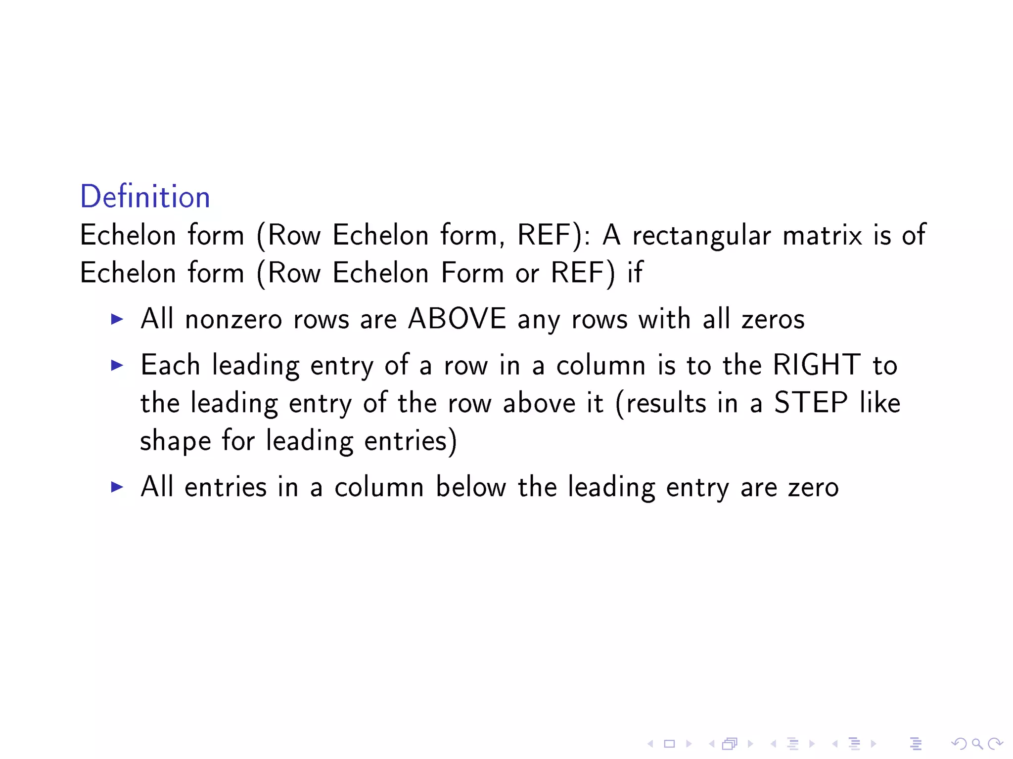
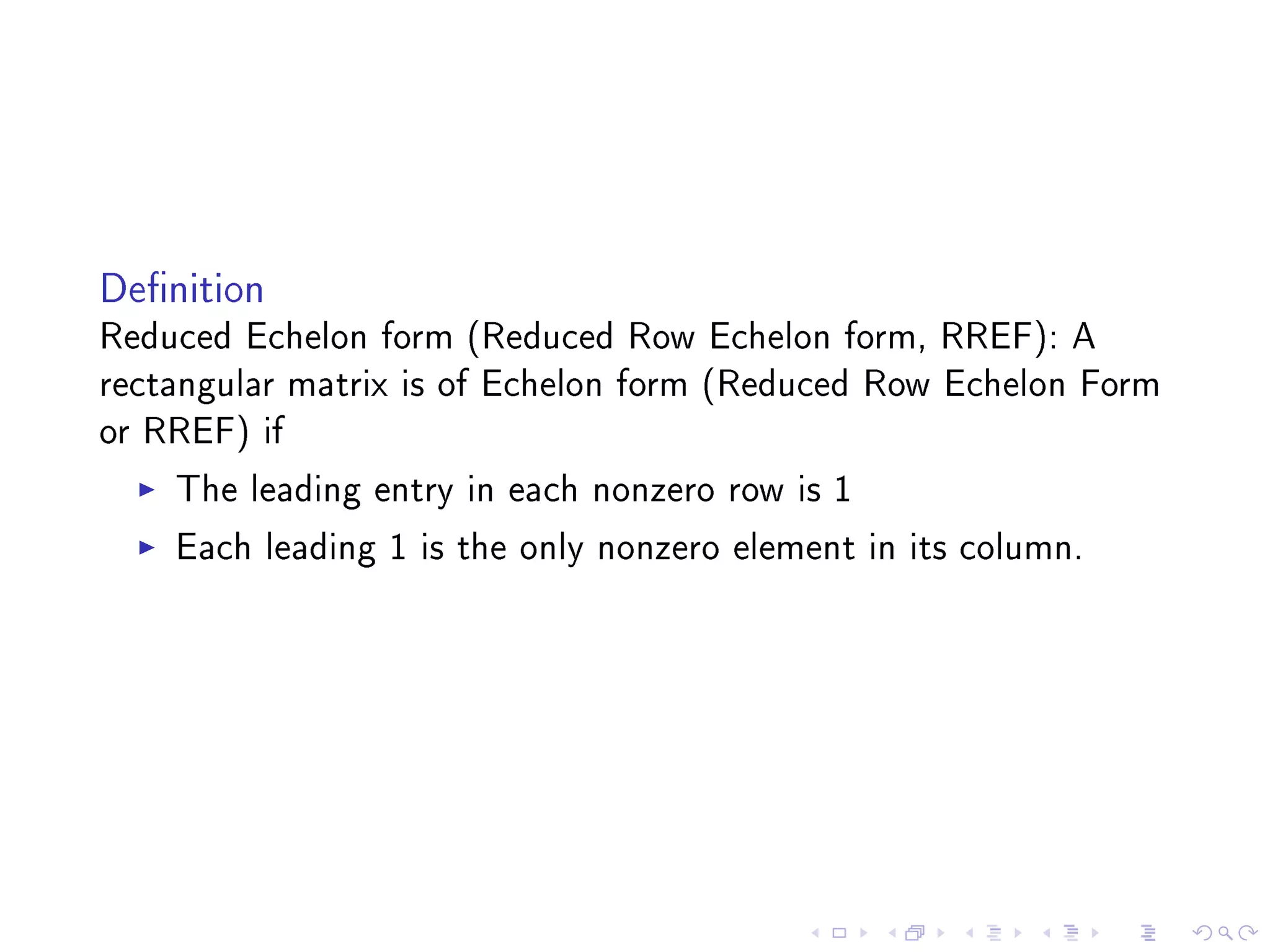
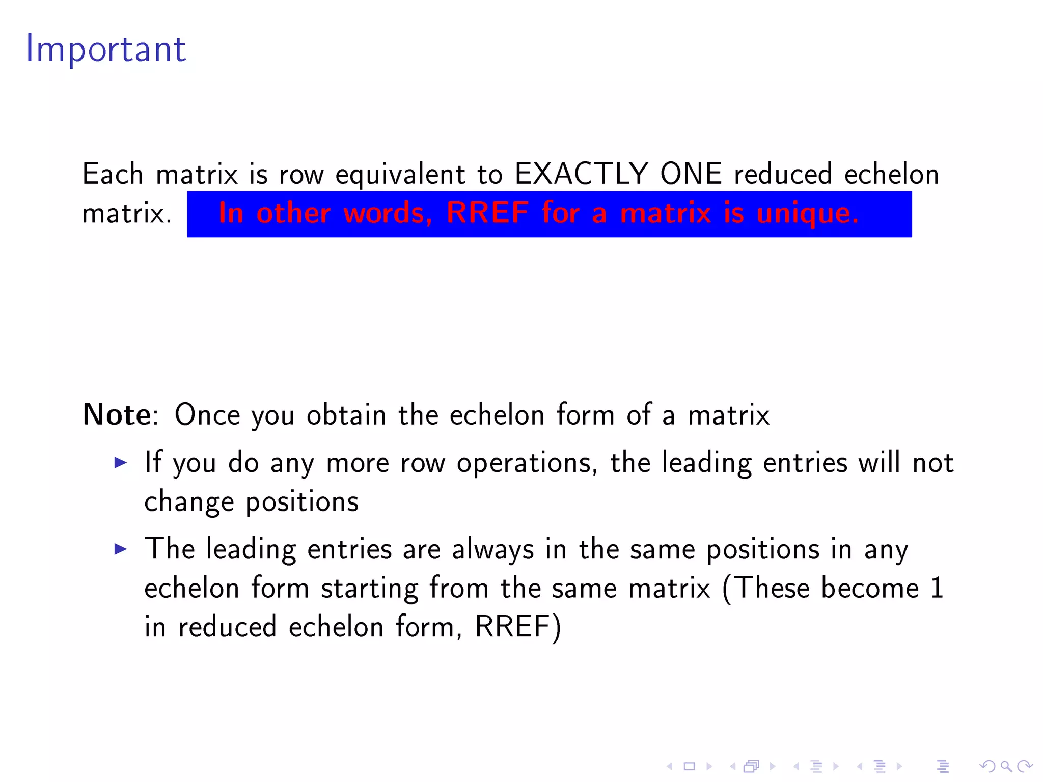
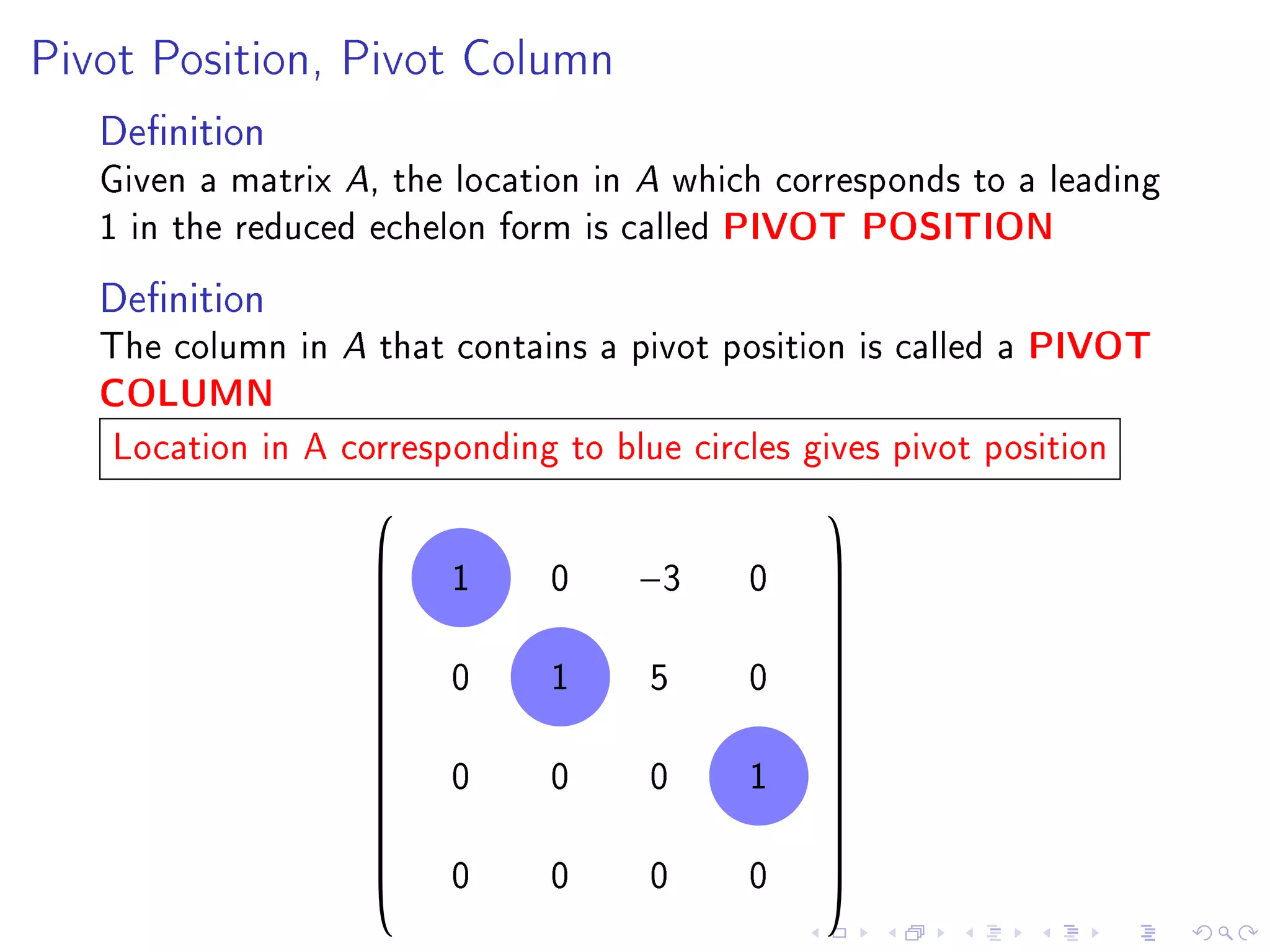
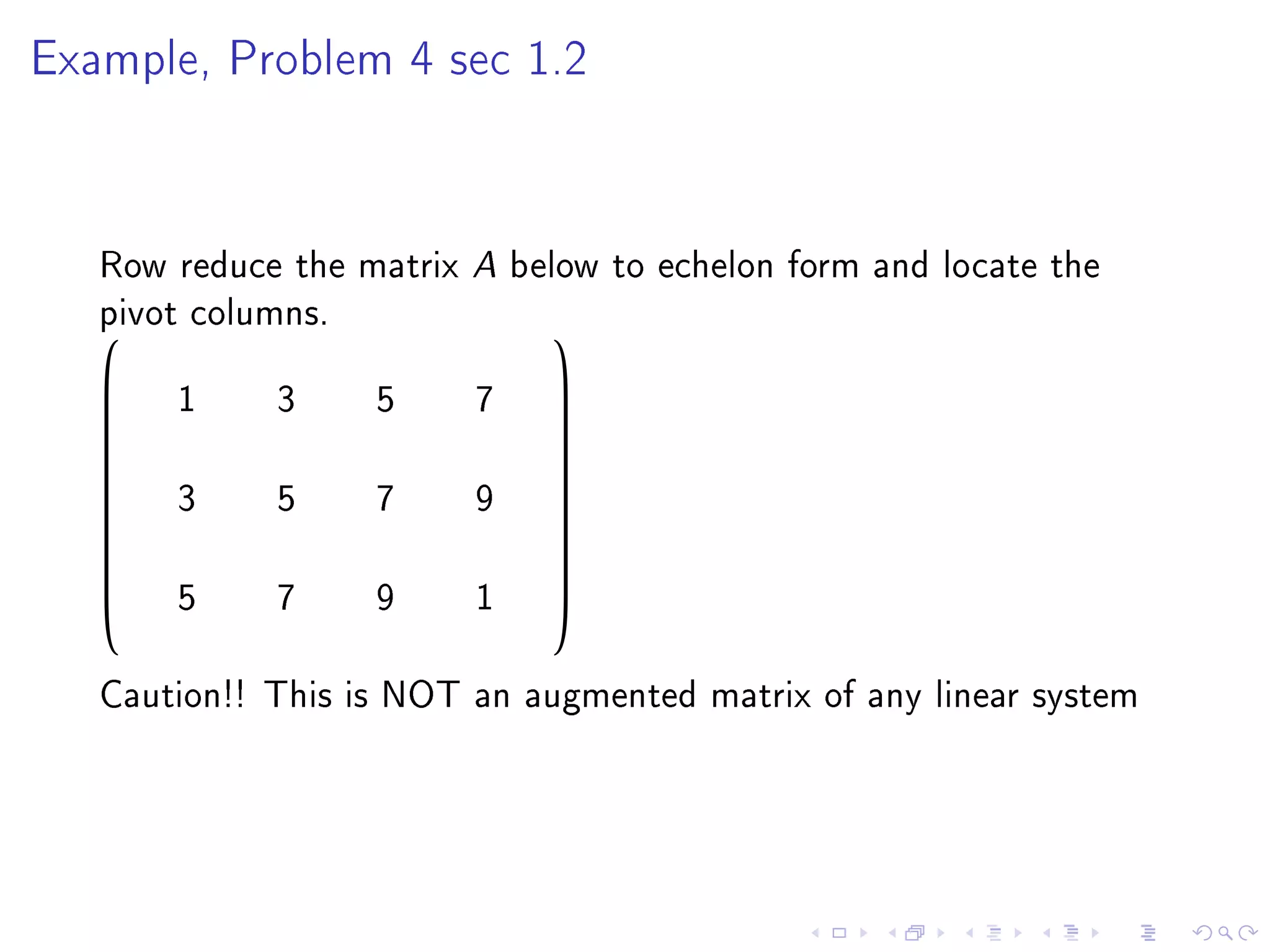
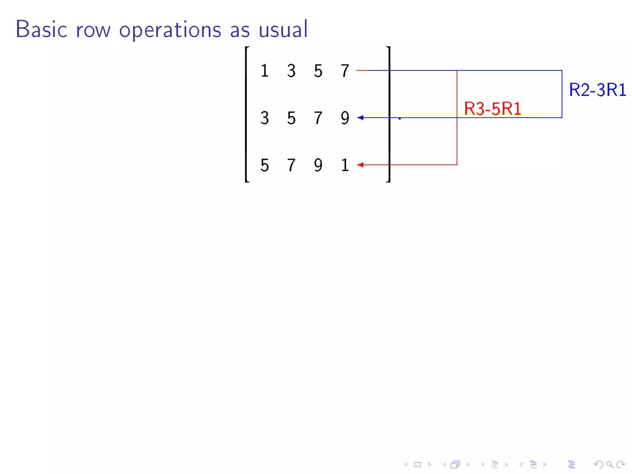
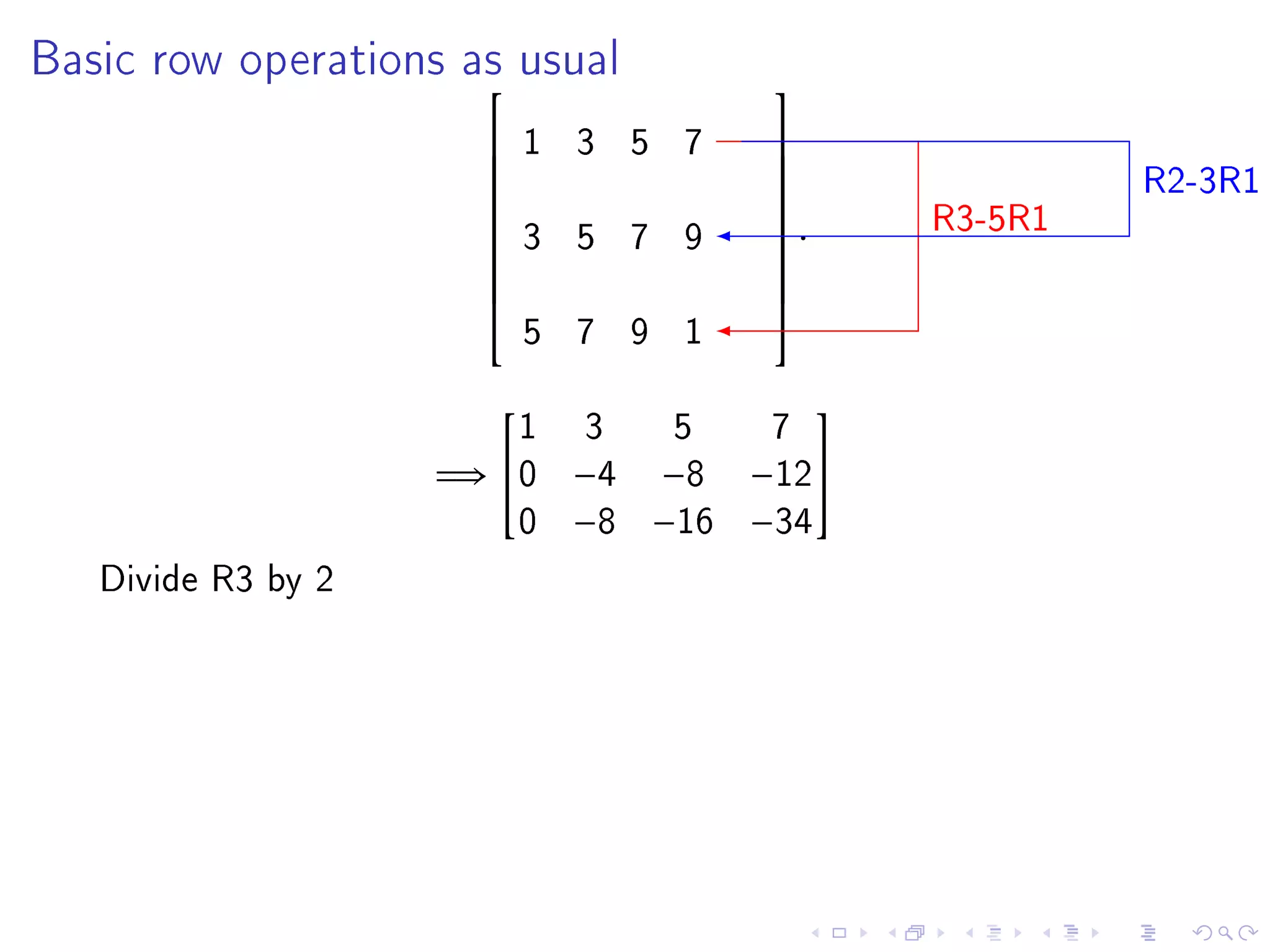
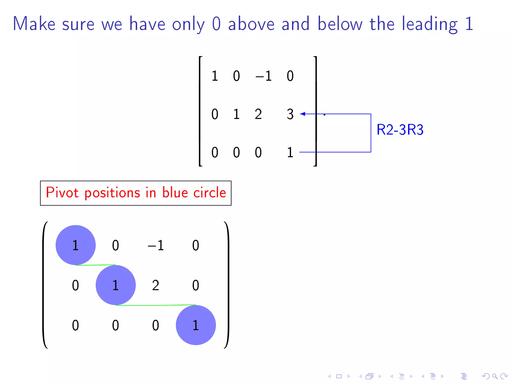
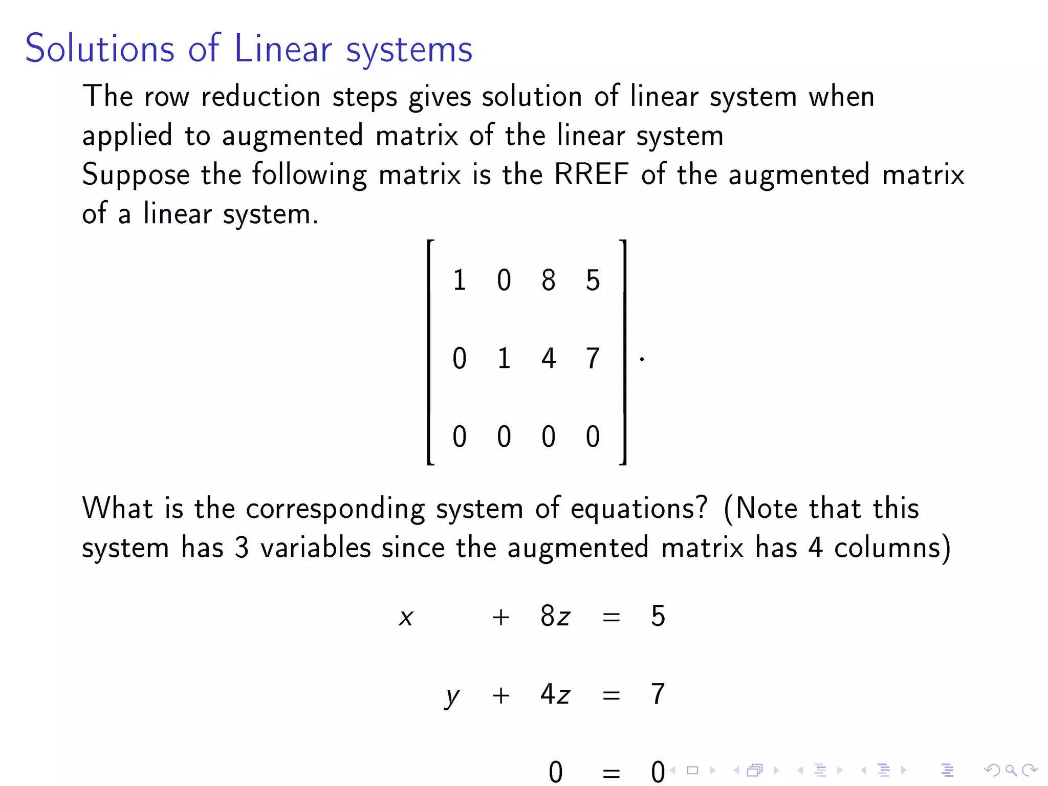
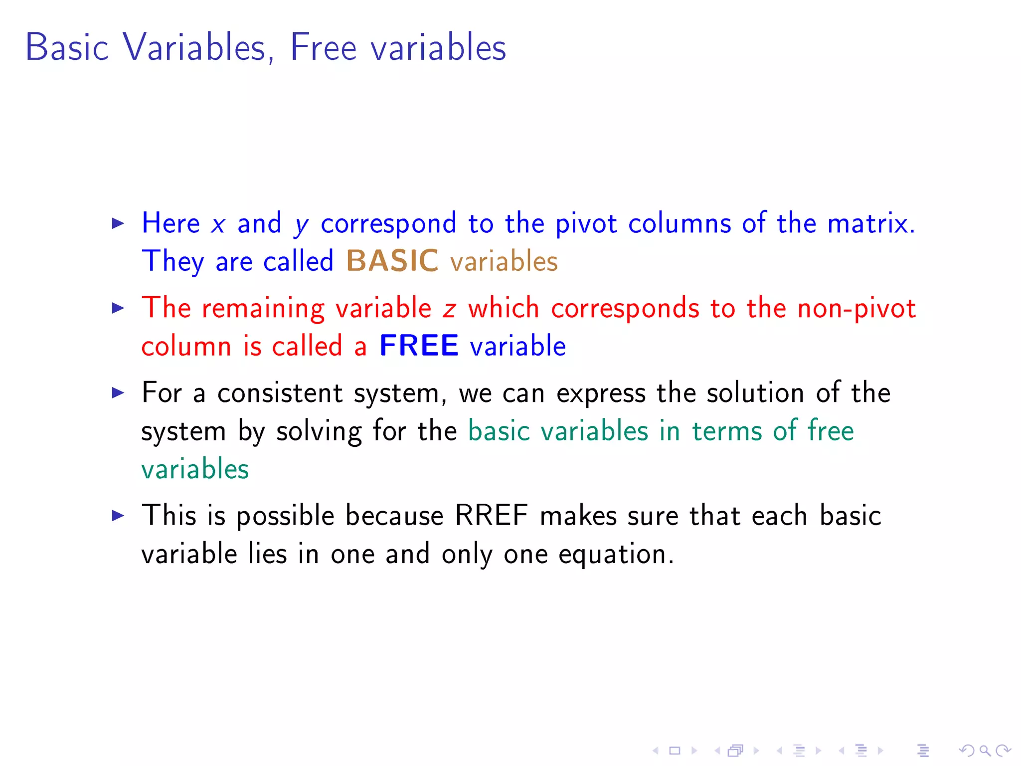
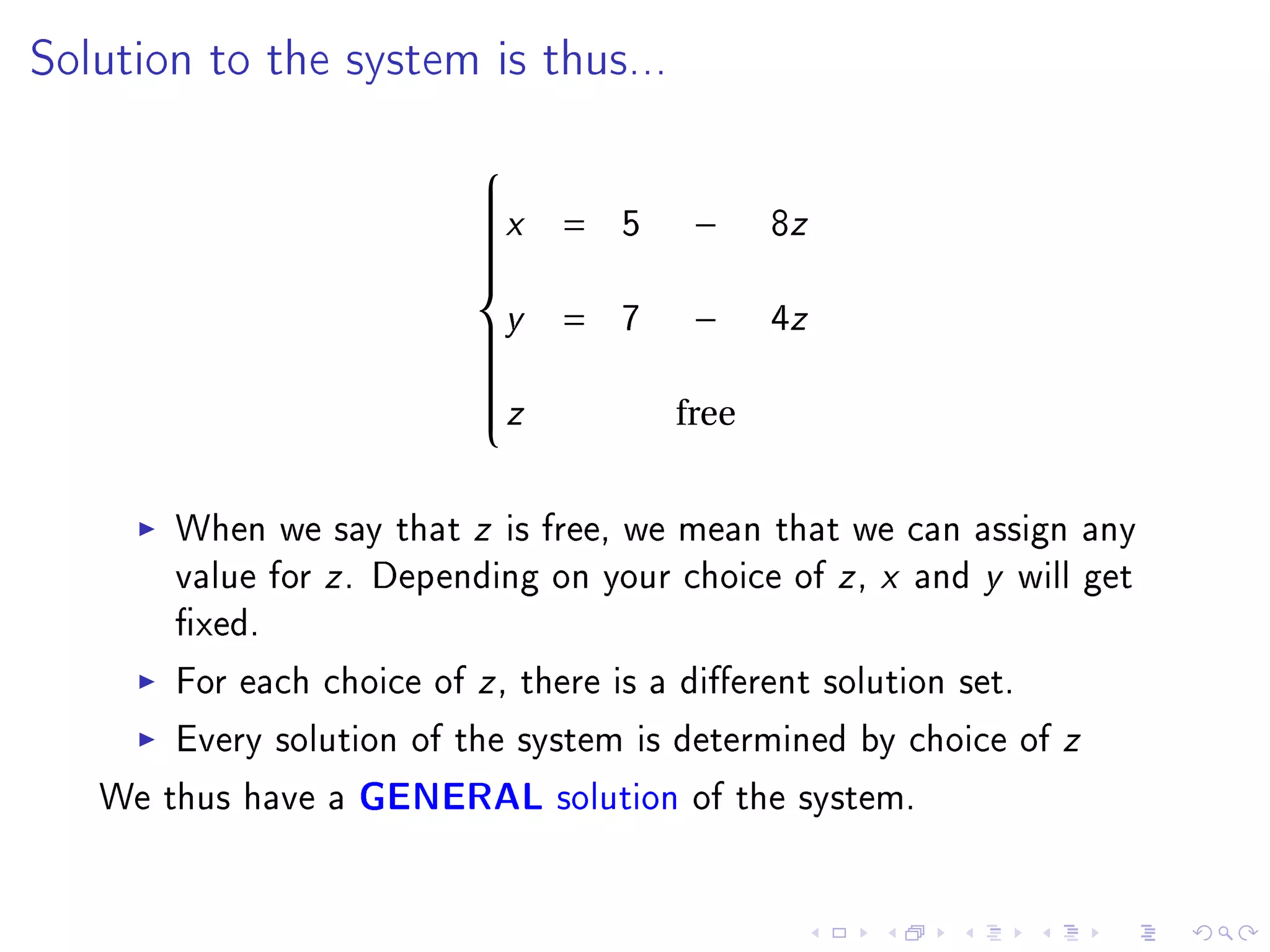
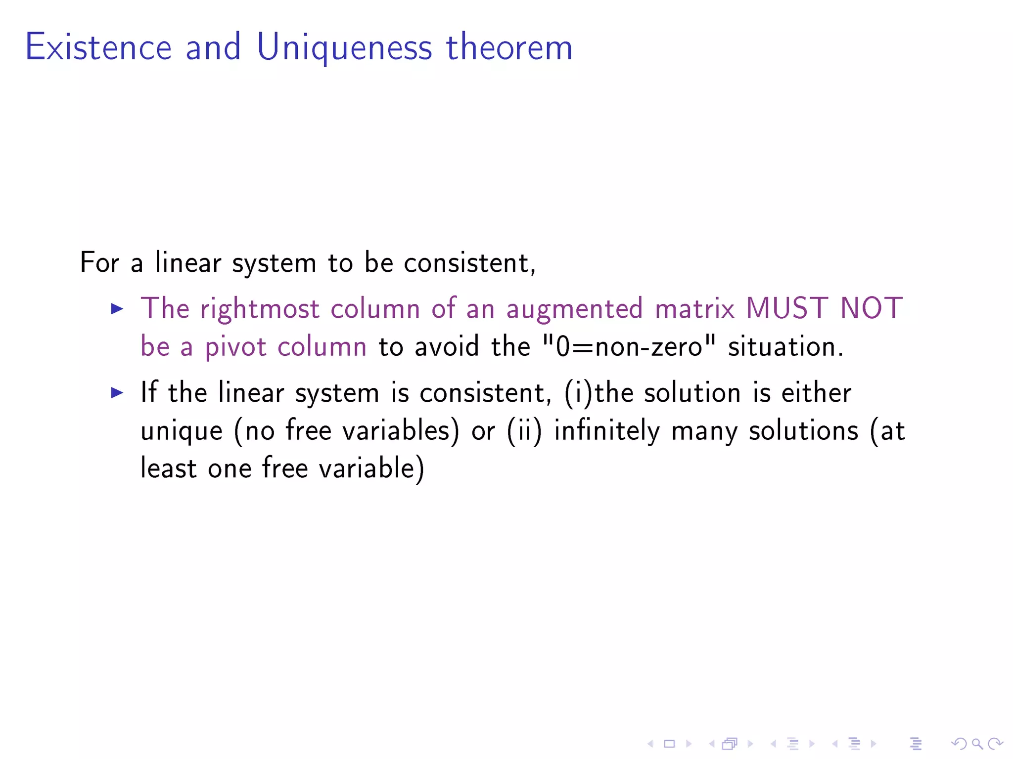
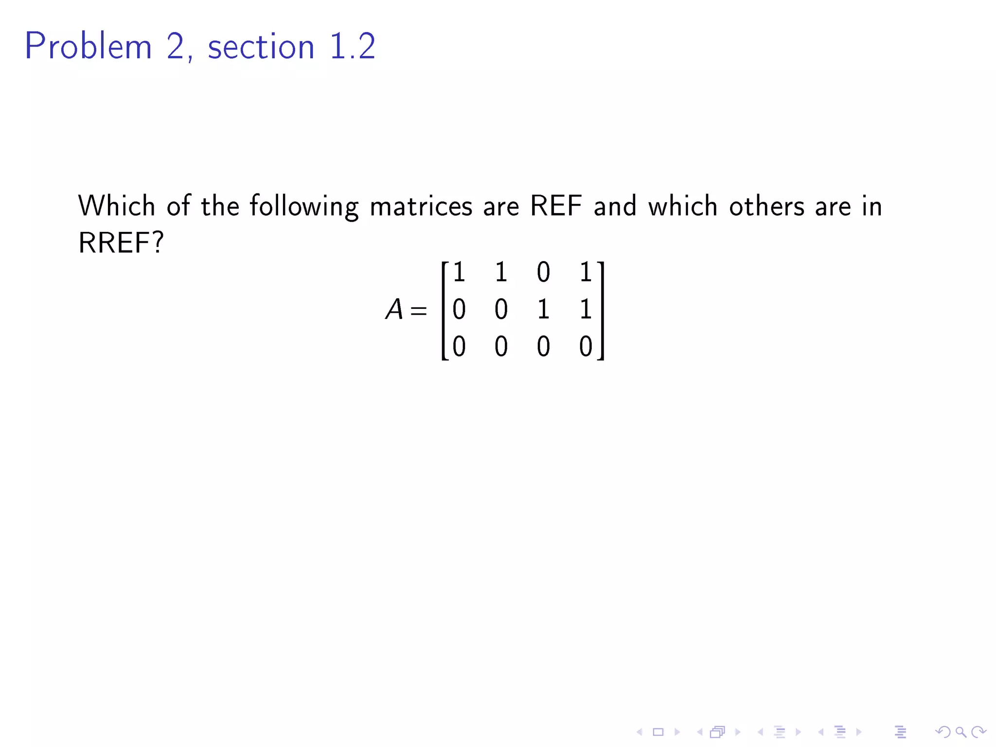
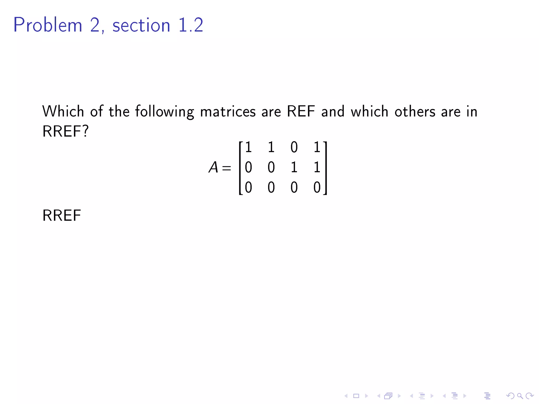
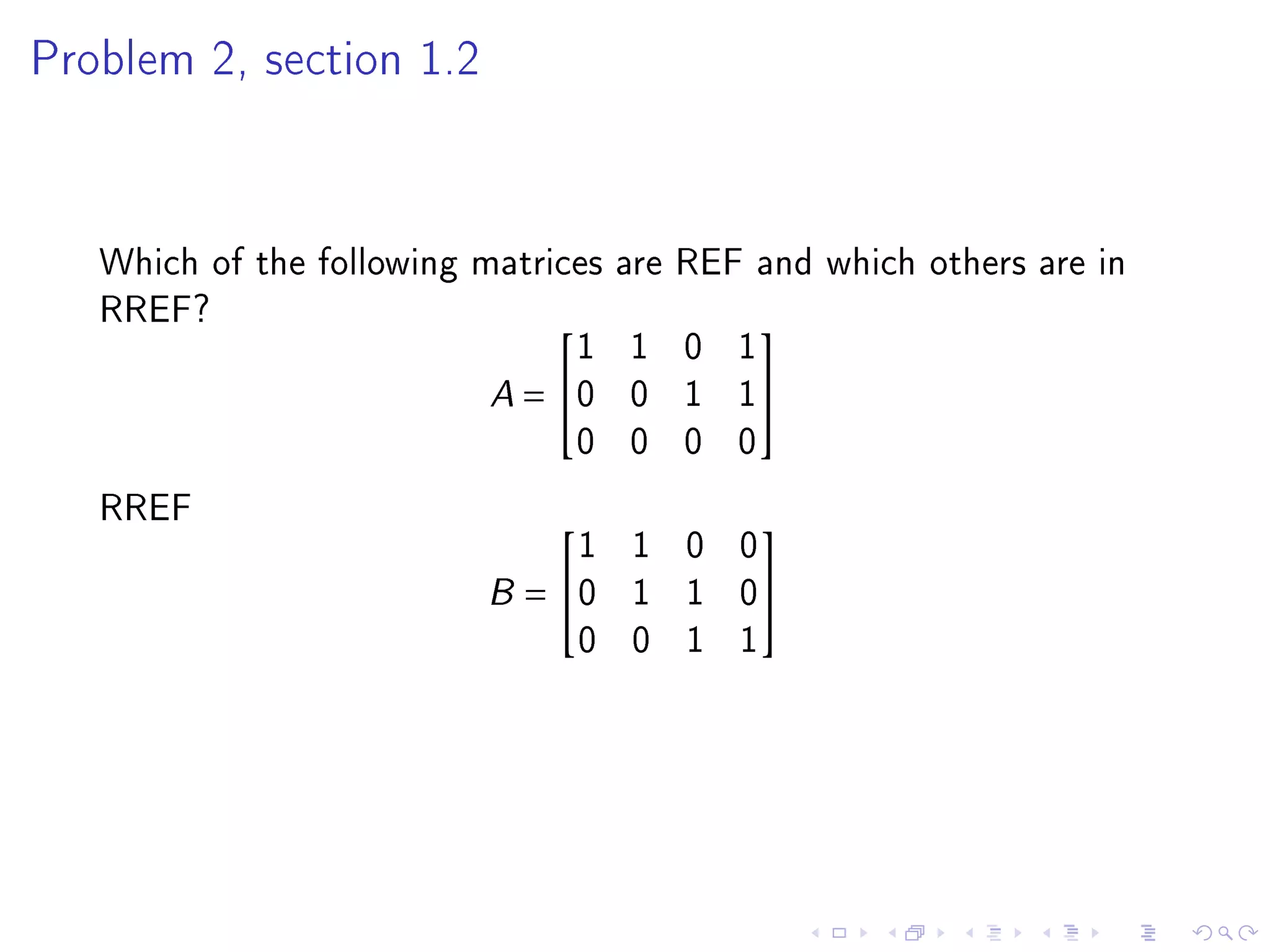
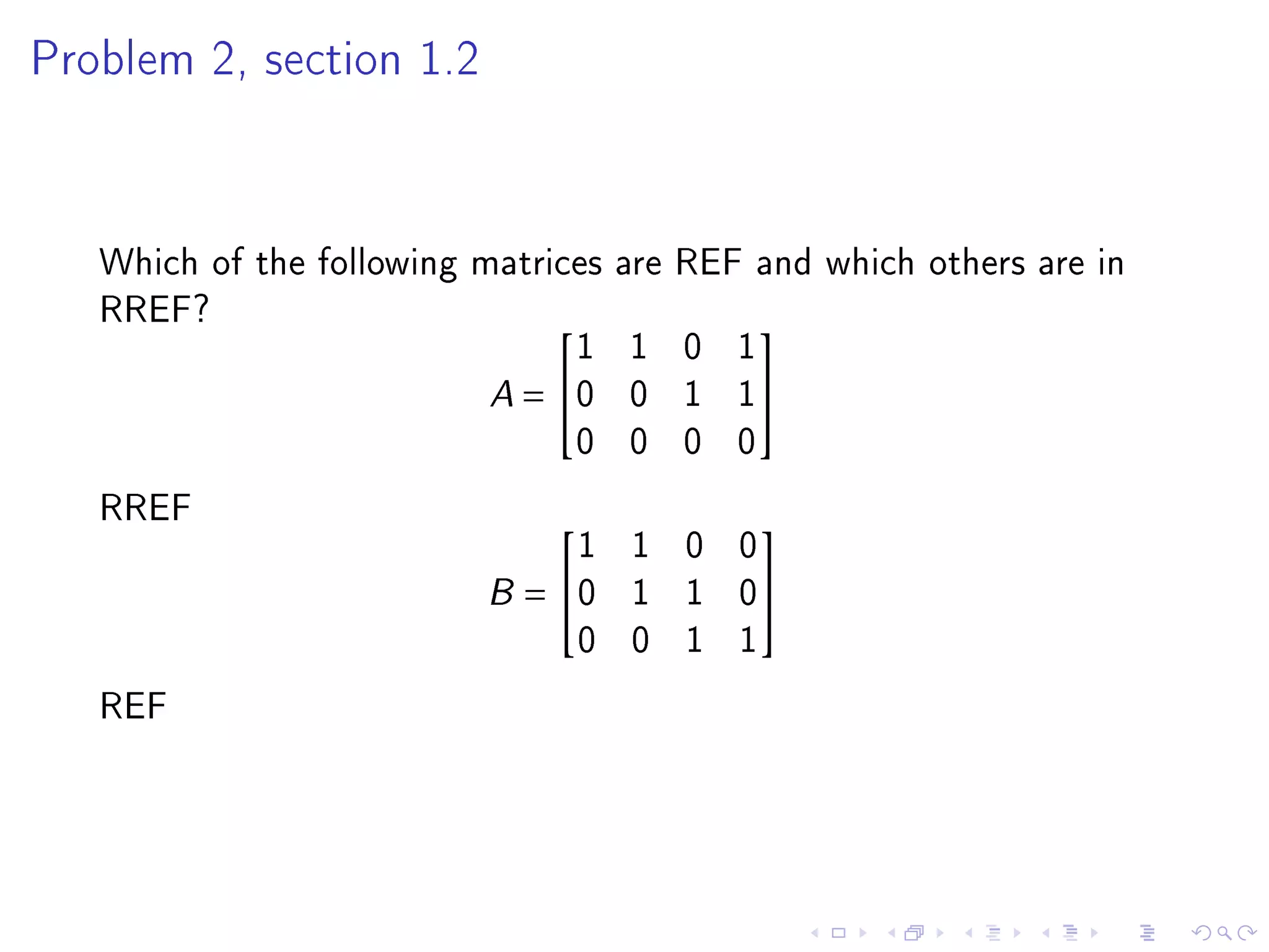
The document contains announcements and information about a class. It announces corrections to lecture slides, the last day to drop the class with a refund, and provides definitions and examples related to echelon form, reduced row echelon form, pivot positions, and solving systems of linear equations.

1. Announcements
If anyone has not been able to access the class website please
email me at pgeorge3@mtu.edu
Two corrections made to Tuesday's lecture slides (Jan 12).
See slides 27, 28 (I had written R3-R1 instead of R3-2R1) and
39 (I didn't make it completely RREF before saving).
If you spot any typos in the slides any time, please bring it to
my attention asap.
Lst day to drop this class with refund is tomorrow.

2. Denition
Echelon form (Row Echelon form, REF): A rectangular matrix is of
Echelon form (Row Echelon Form or REF) if
All nonzero rows are ABOVE any rows with all zeros
Each leading entry of a row in a column is to the RIGHT to
the leading entry of the row above it (results in a STEP like
shape for leading entries)
All entries in a column below the leading entry are zero

3. Denition
Reduced Echelon form (Reduced Row Echelon form, RREF): A
rectangular matrix is of Echelon form (Reduced Row Echelon Form
or RREF) if
The leading entry in each nonzero row is 1
Each leading 1 is the only nonzero element in its column.

4. Important
Each matrix is row equivalent to EXACTLY ONE reduced echelon
matrix. In other words, RREF for a matrix is unique.
Note: Once you obtain the echelon form of a matrix
If you do any more row operations, the leading entries will not
change positions
The leading entries are always in the same positions in any
echelon form starting from the same matrix (These become 1
in reduced echelon form, RREF)

5. Pivot Position, Pivot Column
Denition
Given a matrix A, the location in A which corresponds to a leading
1 in the reduced echelon form is called PIVOT POSITION
Denition
The column in A that contains a pivot position is called a PIVOT
COLUMN
Location in A corresponding to blue circles gives pivot position
 

 1 0 −3 0 

 
 
0 1 5 0
 
 
 
 
 

 0 0 0 1 

 
 
0 0 0 0
 
 

6. Example, Problem 4 sec 1.2
Row reduce the matrix A below to echelon form and locate the
pivot columns.
 

 1 3 5 7 

 
 
3 5 7 9
 
 
 
 
5 7 9 1
 
 
Caution!! This is NOT an augmented matrix of any linear system

7. Basic row operations as usual
 
1 3 5 7
R2-3R1
 
 
R3-5R1
 
3 5 7 9 .
 

 
 
5 7 9 1
 

8. Basic row operations as usual
 
1 3 5 7
R2-3R1
 
 
R3-5R1
 
3 5 7 9 .
 

 
 
5 7 9 1
 
1 3 5 7
 
=⇒ 0 −4 −8 −12
0 −8 −16 −34
Divide R3 by 2

9. Basic row operations as usual
 
1 3 5 7
R2-3R1
 
 
R3-5R1
 
3 5 7 9 .
 

 
 
5 7 9 1
 
1 3 5 7
 
=⇒ 0 −4 −8 −12
0 −8 −16 −34
Divide R3 by 2
1 3 5 7
 
0 −4 −8 −12
0 −4 −8 −17
Do R3-R2

10. Basic row operations as usual
 
1 3 5 7
R2-3R1
 
 
R3-5R1
 
3 5 7 9 .
 

 
 
5 7 9 1
 
1 3 5 7
 
=⇒ 0 −4 −8 −12
0 −8 −16 −34
Divide R3 by 2
1 3 5 7
 
0 −4 −8 −12
0 −4 −8 −17
Do R3-R2
1 3 5 7
 
0 −4 −8 −12
0 0 0 −5

11. Make sure we have only 0 above and below the leading 1
Divide R2 by -4 and divide R3 by -5 to get 1 as leading term. This
gives

12. Make sure we have only 0 above and below the leading 1
Divide R2 by -4 and divide R3 by -5 to get 1 as leading term. This
gives
1 3 5 7
 
0 1 2 3
0 0 0 1
 
1 3 5 7
R1-3R2
 
 
 
0 1 2 3 .
 

 
 
0 0 0 1
 

13. Make sure we have only 0 above and below the leading 1
Divide R2 by -4 and divide R3 by -5 to get 1 as leading term. This
gives
1 3 5 7
 
0 1 2 3
0 0 0 1
 
1 3 5 7
R1-3R2
 
 
 
0 1 2 3 .
 

 
 
0 0 0 1
 
1 0 −1 −2
 
=⇒ 0 1 2 3
0 0 0 1

14. Make sure we have only 0 above and below the leading 1
 
 1 0 −1 −2 
 
R1+2R3
 
0 1 2 3 .
 

 
 
0 0 0 1
 

15. Make sure we have only 0 above and below the leading 1
 
 1 0 −1 −2 
 
R1+2R3
 
0 1 2 3 .
 

 
 
0 0 0 1
 
1 0 −1 0
 
=⇒ 0 1 2 3
0 0 0 1

16. Make sure we have only 0 above and below the leading 1
 
 1 0 −1 0 
 
 
0 1 2 3 .
 

R2-3R3
 
 
0 0 0 1
 

17. Make sure we have only 0 above and below the leading 1
 
 1 0 −1 0 
 
 
0 1 2 3 .
 

R2-3R3
 
 
0 0 0 1
 
Pivot positions in blue circle
 

 1 0 −1 0 

 
 
0 1 2 0
 
 
 
 
0 0 0 1
 
 

18. Answer
We have pivot positions at the blue circles
We need to nd the pivot columns

19. Answer
We have pivot positions at the blue circles
We need to nd the pivot columns
These are the corresponding columns in the original matrix,
that is Column 1, Column 2 and Column 4 in A (not the
columns in RREF)

20. Solutions of Linear systems
The row reduction steps gives solution of linear system when
applied to augmented matrix of the linear system

21. Solutions of Linear systems
The row reduction steps gives solution of linear system when
applied to augmented matrix of the linear system
Suppose the following matrix is the RREF of the augmented matrix
of a linear system.  
 1 0 8 5 
 
 
0 1 4 7 .
 

 
 
0 0 0 0
 
What is the corresponding system of equations? (Note that this
system has 3 variables since the augmented matrix has 4 columns)
x + 8z = 5
y + 4z = 7
0 = 0

22. Basic Variables, Free variables
Here x and y correspond to the pivot columns of the matrix.
They are called BASIC variables
The remaining variable z which corresponds to the non-pivot
column is called a FREE variable
For a consistent system, we can express the solution of the
system by solving for the basic variables in terms of free
variables
This is possible because RREF makes sure that each basic
variable lies in one and only one equation.

23. Solution to the system is thus...

x 5 8z

= −






y

= 7 − 4z


z


free

When we say that z is free, we mean that we can assign any
value for z . Depending on your choice of z , x and y will get
xed.
For each choice of z , there is a dierent solution set.
Every solution of the system is determined by choice of z
We thus have a GENERAL solution of the system.

24. Existence and Uniqueness theorem
For a linear system to be consistent,
The rightmost column of an augmented matrix MUST NOT
be a pivot column to avoid the 0=non-zero situation.
If the linear system is consistent, (i)the solution is either
unique (no free variables) or (ii) innitely many solutions (at
least one free variable)

25. Problem 2, section 1.2
Which of the following matrices are REF and which others are in
RREF?
1 1 0 1
 
A = 0 0 1 1
0 0 0 0

26. Problem 2, section 1.2
Which of the following matrices are REF and which others are in
RREF?
1 1 0 1
 
A = 0 0 1 1
0 0 0 0
RREF

27. Problem 2, section 1.2
Which of the following matrices are REF and which others are in
RREF?
1 1 0 1
 
A = 0 0 1 1
0 0 0 0
RREF
1 1 0 0
 
B= 0 1 1 0
0 0 1 1

28. Problem 2, section 1.2
Which of the following matrices are REF and which others are in
RREF?
1 1 0 1
 
A = 0 0 1 1
0 0 0 0
RREF
1 1 0 0
 
B= 0 1 1 0
0 0 1 1
REF

29. Problem 2, section 1.2
Which of the following matrices are REF and which others are in
RREF?
1 0 0 0
 
A = 1 1 0 0
 
0 1 1 0
 
0 0 1 1

30. Problem 2, section 1.2
Which of the following matrices are REF and which others are in
RREF?
1 0 0 0
 
A = 1 1 0 0
 
0 1 1 0
 
0 0 1 1
Neither (The leading element in a row must be to the right of the
leading element in the row above, no step pattern)

31. Problem 2, section 1.2
Which of the following matrices are REF and which others are in
RREF?
1 0 0 0
 
A = 1 1 0 0
 
0 1 1 0
 
0 0 1 1
Neither (The leading element in a row must be to the right of the
leading element in the row above, no step pattern)
0 1 1 1 1
 
0 0 2 2 2
B = 0

 0 0 0 3


0 0 0 0 0

32. Problem 2, section 1.2
Which of the following matrices are REF and which others are in
RREF?
1 0 0 0
 
A = 1 1 0 0
 
0 1 1 0
 
0 0 1 1
Neither (The leading element in a row must be to the right of the
leading element in the row above, no step pattern)
0 1 1 1 1
 
0 0 2 2 2
B = 0

 0 0 0 3


0 0 0 0 0
REF

33. Problem 12, section 1.2
Find the general solutions of the systems whose augmented matrix
is given below
1 −7 0 6 5
 
A =  0 0 1 −2 −3
−1 7 −4 2 7

34. Problem 12, section 1.2
Find the general solutions of the systems whose augmented matrix
is given below
1 −7 0 6 5
 
A =  0 0 1 −2 −3
−1 7 −4 2 7
Do R3+R1 to get new R3
1 −7 0 6 5
 
B= 0 0 1 −2 −3
0 0 −4 8 12

35. Problem 12, section 1.2
Find the general solutions of the systems whose augmented matrix
is given below
1 −7 0 6 5
 
A =  0 0 1 −2 −3
−1 7 −4 2 7
Do R3+R1 to get new R3
1 −7 0 6 5
 
B= 0 0 1 −2 −3
0 0 −4 8 12
Divide last row by -4
1 −7 0 6 5
 
B = 0 0 1 −2 −3
0 0 1 −2 −3

36. Problem 12, section 1.2
Do R3-R2 to get new R3
1 −7 0 6 5
 
B= 0 0 1 −2 −3
0 0 0 0 0
Our system of equations thus is
x1 − 7x2 + 6x4 = 5
x3 − 2x4 = −3
0 = 0
Column 1 and Column 3 have the pivot positions. The
corresponding variables x1 and x3 are basic variables. So, x2 and x4
are free variables.

37. Problem 12, section 1.2
To get the general solution, express the basic variables in terms of
the free variables. This gives

x1 5 6x4 7x2

= − +






x3

= −3 + 2x4


x2 x4


and free


38. Problem 20, section 1.2
Choose h and k such that the system has (a) no solution (b)
exactly one solution and (c) innitely many solutions
x1 + 3x2 = 2
3x1 + hx2 = k
Solution: As usual, start with the augmented matrix
 

 1 3 2 

 
h k
 

3 

39. Problem 20, section 1.2
 
 1 3 2 

 .

R2-3R1
3 h k
 

40. Problem 20, section 1.2
 
 1 3 2 

 .

R2-3R1
3 h k
 
1 3 2
0 h−9 k −6
If h = 9 AND k = 6, we have 0=0 which means there is a free
variable. So innite number of solutions for this choice.
If h = 9 and k = 6 we have 0=non-zero situation. So
inconsistent for this choice of h and k .
If h = 9 and for any value of k we have exactly one solution.

41. Section 1.3, Vector Equations
A vector is nothing but a list of numbers (for the time being).
1
In the 2 dimensional x − y plane, this will look like u= or
2
v= −52 or w= .52 .1
Such a matrix with only 1 column is called a column vector or
just vector
Adding (or subtracting) 2 vectors is easy, just subtract the
1 6
corresponding entries. So if u= and v= then
4 −2
u+v= 1 + 6 = 7
4−2 2
You can multiply a vector with a number, it scales the vector
1 5
accordingly. So if u= then 5u=
4 20

42. Some Geometry
a
The column vector =
b identies the point (a,b) on the x − y
plane
3
The vector u= is an arrow from the origin (0,0) to (3,2)
2

43. Some Geometry
a
The column vector =
b identies the point (a,b) on the x − y
plane
3
The vector u= is an arrow from the origin (0,0) to (3,2)
2
y
(3, 2)
(0, 0) x

44. Some Geometry
a
The column vector =
b identies the point (a,b) on the x − y
plane
3
The vector u= is an arrow from the origin (0,0) to (3,2)
2
y
(3, 2)
(0, 0) x

45. Some Geometry
a
The column vector =
b identies the point (a,b) on the x − y
plane
3
The vector u= is an arrow from the origin (0,0) to (3,2)
2
y
(3, 2)
(-2, 1)
(0, 0) x

46. Some Geometry
a
The column vector =
b identies the point (a,b) on the x − y
plane
3
The vector u= is an arrow from the origin (0,0) to (3,2)
2
y
(3, 2)
(-2, 1)
(0, 0) x

47. Parallelogram rule for vector addition
If u and v are points in a plane, then u+v is the fourth vertex of a
parallelogram whose other vertices are u, 0 and v

48. Parallelogram rule for vector addition
If u and v are points in a plane, then u+v is the fourth vertex of a
parallelogram whose other vertices are u, 0 and v
y
u
x
0

49. Parallelogram rule for vector addition
If u and v are points in a plane, then u+v is the fourth vertex of a
parallelogram whose other vertices are u, 0 and v
y
u
x
0

50. Parallelogram rule for vector addition
If u and v are points in a plane, then u+v is the fourth vertex of a
parallelogram whose other vertices are u, 0 and v
y
v
u
x
0

51. Parallelogram rule for vector addition
If u and v are points in a plane, then u+v is the fourth vertex of a
parallelogram whose other vertices are u, 0 and v
y
v
u
x
0

52. Parallelogram rule for vector addition
If u and v are points in a plane, then u+v is the fourth vertex of a
parallelogram whose other vertices are u, 0 and v
y u+v
v
u
x
0

53. Parallelogram rule for vector addition
If u and v are points in a plane, then u+v is the fourth vertex of a
parallelogram whose other vertices are u, 0 and v
y u+v
v
u
x
0

54. Parallelogram rule for vector addition
If u and v are points in a plane, then u+v is the fourth vertex of a
parallelogram whose other vertices are u, 0 and v
y u+v
v
u
x
0

55. Scalar Multiplication
Multiplying a vector by a number scales it correspondingly.

56. Scalar Multiplication
Multiplying a vector by a number scales it correspondingly.
y
u
x
0

57. Scalar Multiplication
Multiplying a vector by a number scales it correspondingly.
y
u
x
0

58. Scalar Multiplication
Multiplying a vector by a number scales it correspondingly.
y
u
0.5u
x
0

59. Scalar Multiplication
Multiplying a vector by a number scales it correspondingly.
y
u
0.5u
x
0

60. Scalar Multiplication
Multiplying a vector by a number scales it correspondingly.
y 2u
u
0.5u
x
0

61. Scalar Multiplication
Multiplying a vector by a number scales it correspondingly.
y 2u
u
0.5u
x
0

62. Vectors in 3-D
2
 
Vectors in the x − y − z plane is a 3X1 column matrix. Here u
= 3
4
is illustrated.

63. Vectors in 3-D
2
 
Vectors in the x − y − z plane is a 3X1 column matrix. Here u
= 3
4
is illustrated.
y
u
x
0
z

64. Vectors in 3-D
2
 
Vectors in the x − y − z plane is a 3X1 column matrix. Here u
= 3
4
is illustrated.
y
u
x
0
z