Downloaded 176 times
![FINDING RUNNING TIME OF AN
ALGORITHM / ANALYZING AN
ALGORITHM
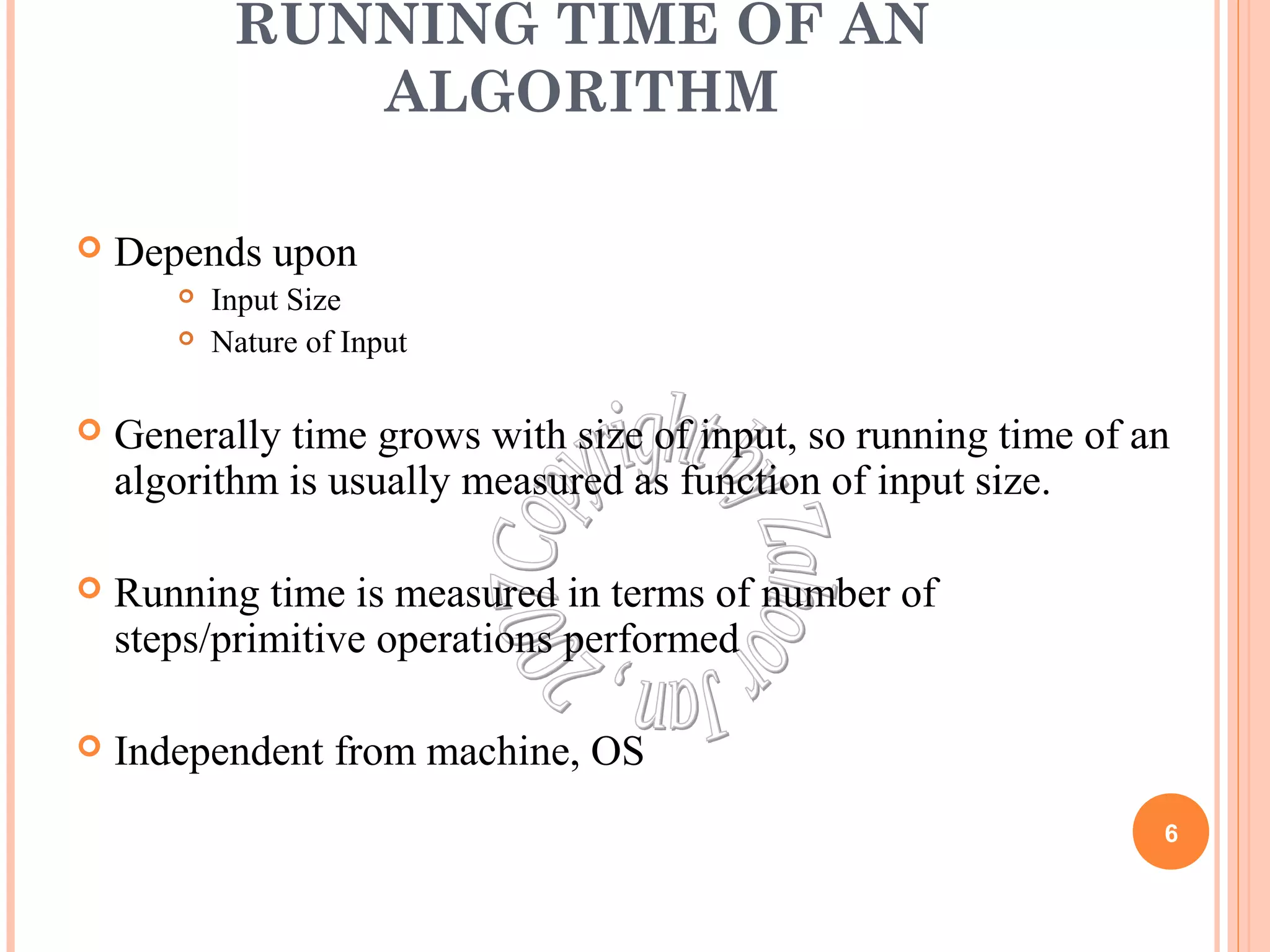
Running time is measured by number of steps/primitive
operations performed
Steps means elementary operation like
,+, *,<, =, A[i] etc
We will measure number of steps taken in term of size of
input
7](https://image.slidesharecdn.com/lec03-04-timecomplexity-141021105349-conversion-gate01/75/Algorithm-And-analysis-Lecture-03-04-time-complexity-7-2048.jpg)
![SIMPLE EXAMPLE (1)
// Input: int A[N], array of N integers
// Output: Sum of all numbers in array A
int Sum(int A[], int N)
{
int s=0;
for (int i=0; i< N; i++)
s = s + A[i];
return s;
}
How should we analyse this?
8](https://image.slidesharecdn.com/lec03-04-timecomplexity-141021105349-conversion-gate01/75/Algorithm-And-analysis-Lecture-03-04-time-complexity-8-2048.jpg)
![SIMPLE EXAMPLE (2)
9
// Input: int A[N], array of N integers
// Output: Sum of all numbers in array A
int Sum(int A[], int N){
int s=0;
for (int i=0; i< N; i++)
s = s + A[i];
return s;
}
1
2 3 4
5 6 7
8
1,2,8: Once
3,4,5,6,7: Once per each iteration
of for loop, N iteration
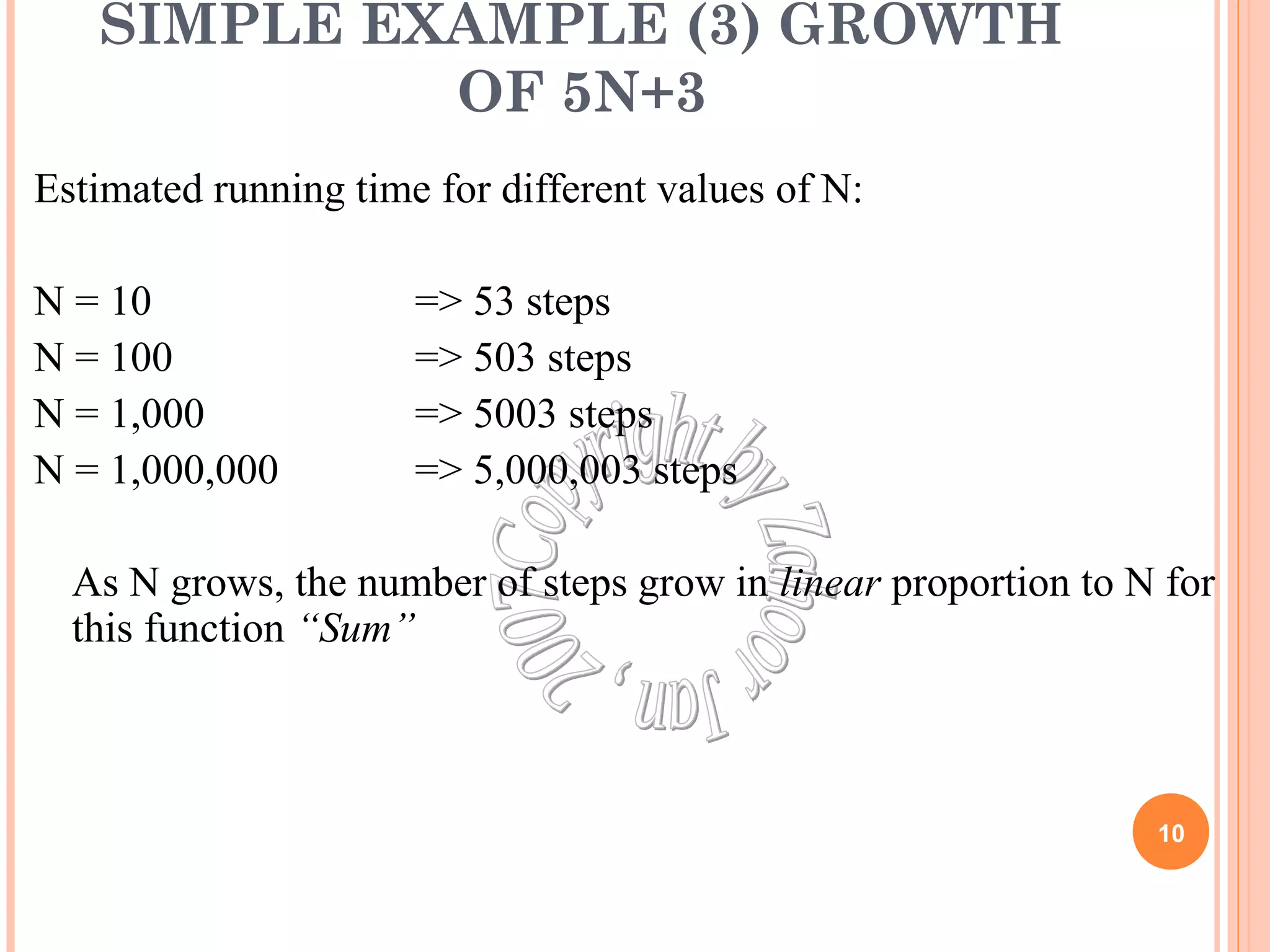
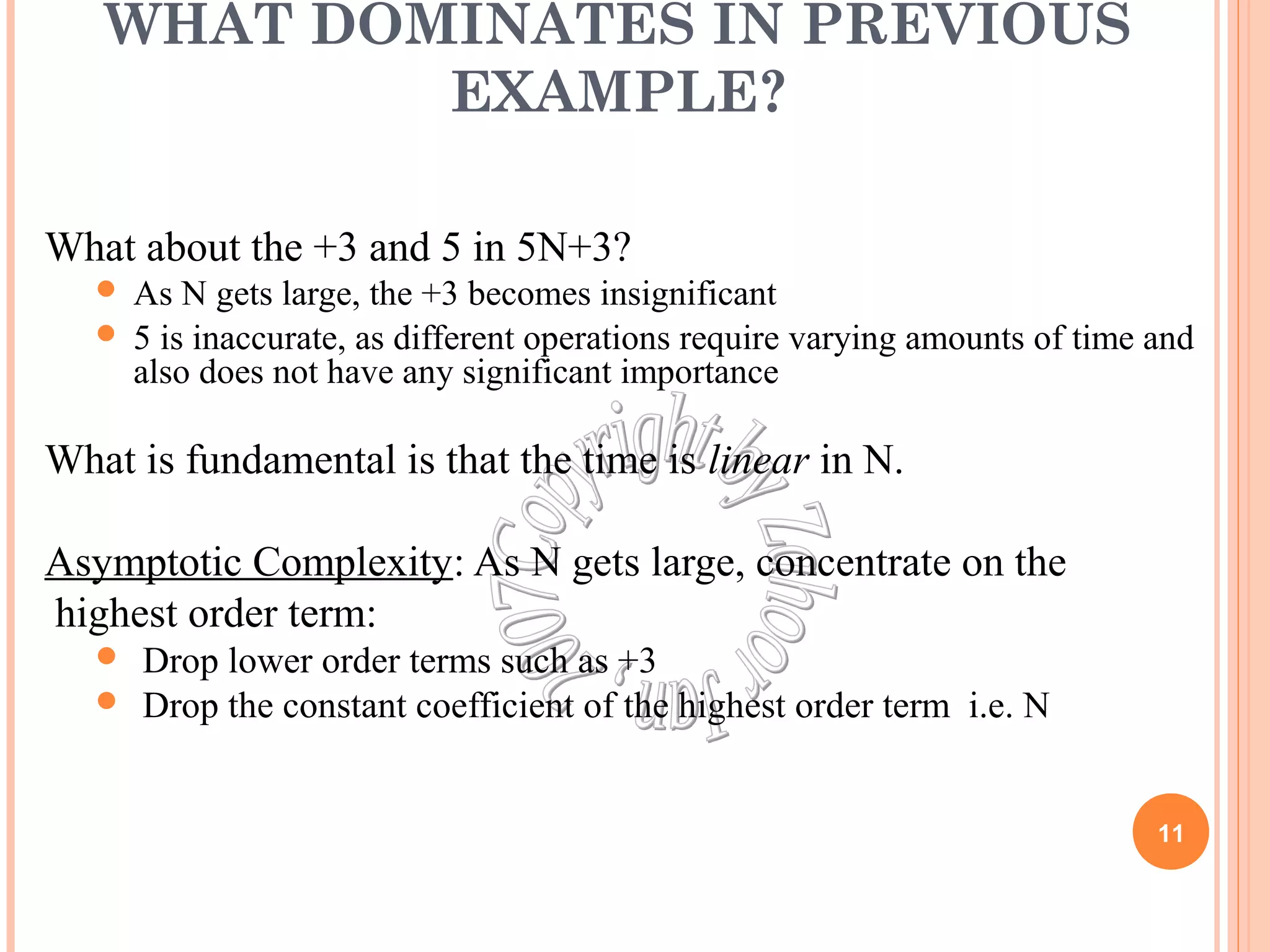
Total: 5N + 3
The complexity function of the
algorithm is : f(N) = 5N +3](https://image.slidesharecdn.com/lec03-04-timecomplexity-141021105349-conversion-gate01/75/Algorithm-And-analysis-Lecture-03-04-time-complexity-9-2048.jpg)
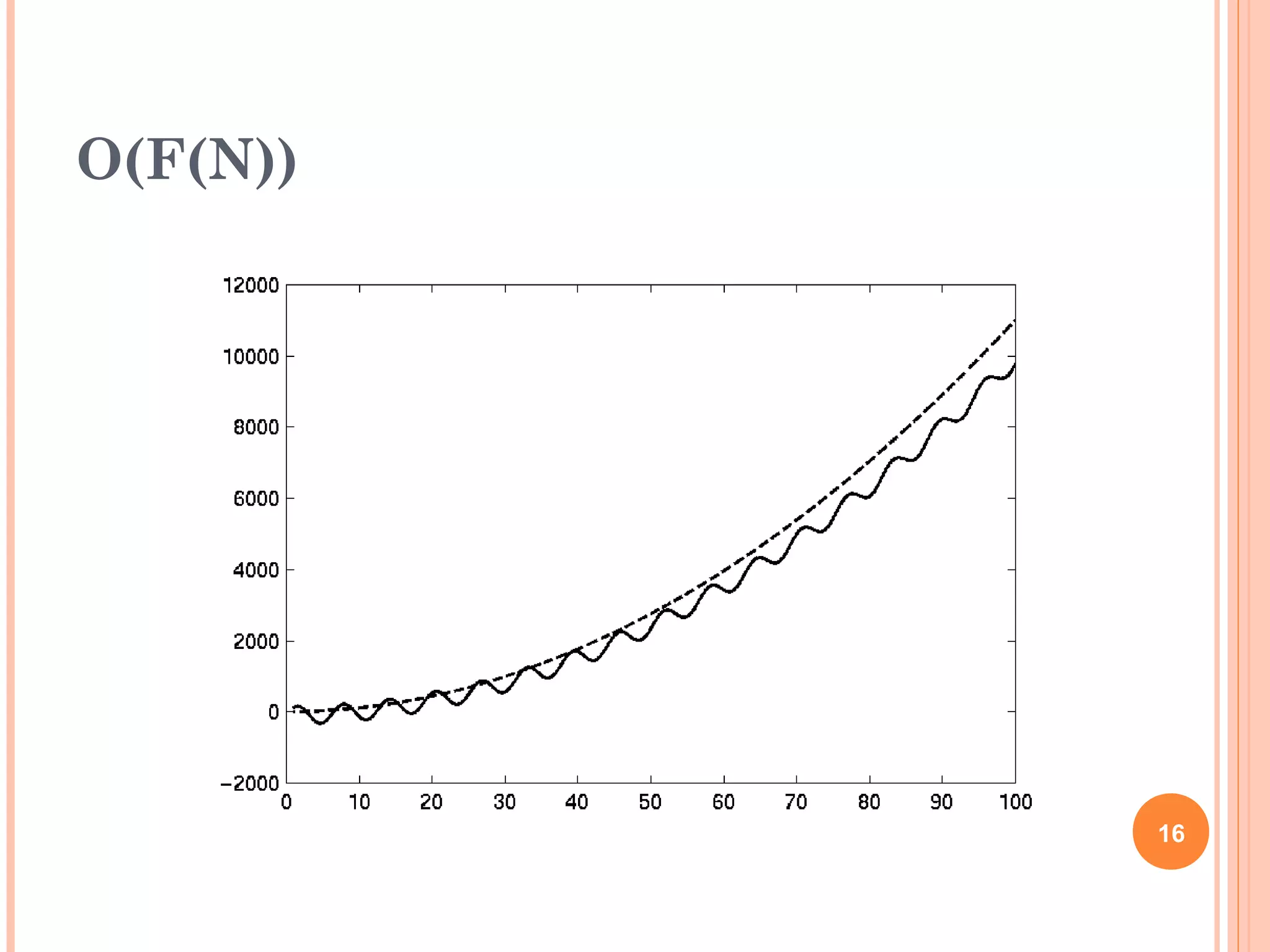
![BIG OH NOTATION [1]
If f(N) and g(N) are two complexity functions, we say
f(N) = O(g(N))
(read "f(N) is order g(N)", or "f(N) is big-O of g(N)")
if there are constants c and N0 such that for N > N0,
f(N) ≤ c * g(N)
for all sufficiently large N.
14](https://image.slidesharecdn.com/lec03-04-timecomplexity-141021105349-conversion-gate01/75/Algorithm-And-analysis-Lecture-03-04-time-complexity-14-2048.jpg)
![BIG OH NOTATION [2]
15](https://image.slidesharecdn.com/lec03-04-timecomplexity-141021105349-conversion-gate01/75/Algorithm-And-analysis-Lecture-03-04-time-complexity-15-2048.jpg)
![SIZE DOES MATTER[1]
25
What happens if we double the input size N?
N log2N 5N N log2N N2 2N
8 3 40 24 64 256
16 4 80 64 256 65536
32 5 160 160 1024 ~109
64 6 320 384 4096 ~1019
128 7 640 896 16384 ~1038
256 8 1280 2048 65536 ~1076](https://image.slidesharecdn.com/lec03-04-timecomplexity-141021105349-conversion-gate01/75/Algorithm-And-analysis-Lecture-03-04-time-complexity-25-2048.jpg)
![SIZE DOES MATTER[2]
Suppose a program has run time O(n!) and the run time for
n = 10 is 1 second
For n = 12, the run time is 2 minutes
For n = 14, the run time is 6 hours
For n = 16, the run time is 2 months
For n = 18, the run time is 50 years
For n = 20, the run time is 200 centuries
27](https://image.slidesharecdn.com/lec03-04-timecomplexity-141021105349-conversion-gate01/75/Algorithm-And-analysis-Lecture-03-04-time-complexity-27-2048.jpg)
![CONSTANT TIME STATEMENTS
Simplest case: O(1) time statements
Assignment statements of simple data types
int x = y;
Arithmetic operations:
x = 5 * y + 4 - z;
Array referencing:
A[j] = 5;
Array assignment:
" j, A[j] = 5;
Most conditional tests:
if (x < 12) ...
29](https://image.slidesharecdn.com/lec03-04-timecomplexity-141021105349-conversion-gate01/75/Algorithm-And-analysis-Lecture-03-04-time-complexity-29-2048.jpg)
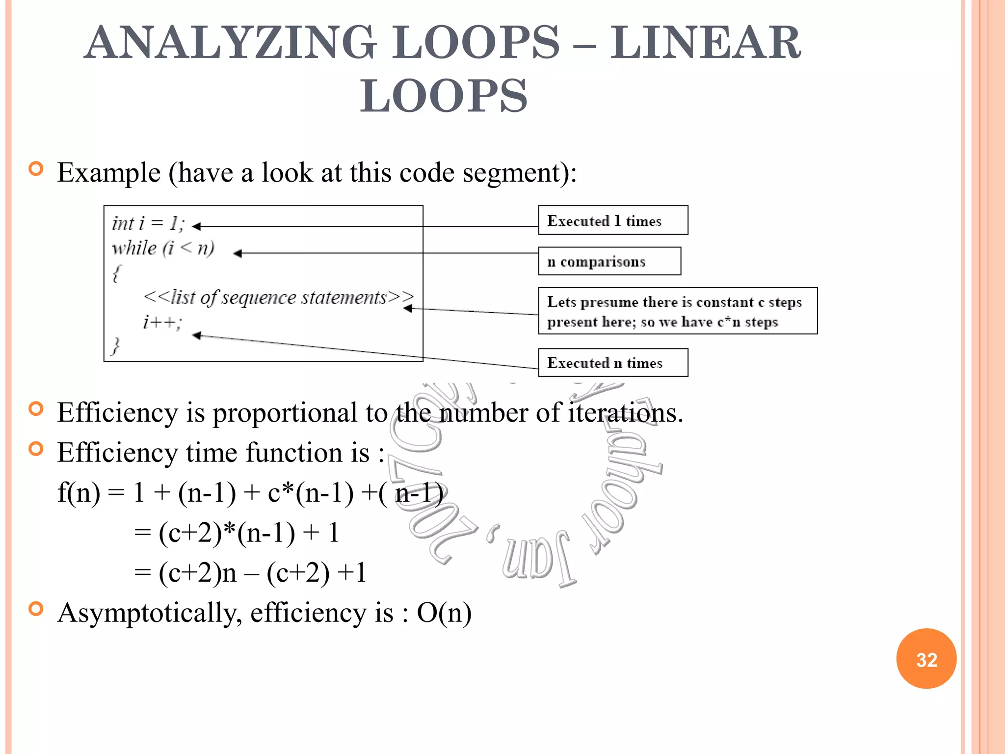
![ANALYZING LOOPS[1]
Any loop has two parts:
How many iterations are performed?
How many steps per iteration?
int sum = 0,j;
for (j=0; j < N; j++)
sum = sum +j;
Loop executes N times (0..N-1)
4 = O(1) steps per iteration
Total time is N * O(1) = O(N*1) = O(N) 30](https://image.slidesharecdn.com/lec03-04-timecomplexity-141021105349-conversion-gate01/75/Algorithm-And-analysis-Lecture-03-04-time-complexity-30-2048.jpg)
![ANALYZING LOOPS[2]
What about this for loop?
int sum =0, j;
for (j=0; j < 100; j++)
sum = sum +j;
Loop executes 100 times
4 = O(1) steps per iteration
Total time is 100 * O(1) = O(100 * 1) = O(100) = O(1)
31](https://image.slidesharecdn.com/lec03-04-timecomplexity-141021105349-conversion-gate01/75/Algorithm-And-analysis-Lecture-03-04-time-complexity-31-2048.jpg)
![ANALYZING NESTED LOOPS[1]
Treat just like a single loop and evaluate each level of nesting as
needed:
int j,k;
for (j=0; j<N; j++)
for (k=N; k>0; k--)
sum += k+j;
Start with outer loop:
How many iterations? N
How much time per iteration? Need to evaluate inner loop
Inner loop uses O(N) time
Total time is N * O(N) = O(N*N) = O(N2) 33](https://image.slidesharecdn.com/lec03-04-timecomplexity-141021105349-conversion-gate01/75/Algorithm-And-analysis-Lecture-03-04-time-complexity-33-2048.jpg)
![ANALYZING NESTED LOOPS[2]
What if the number of iterations of one loop depends on the
counter of the other?
int j,k;
for (j=0; j < N; j++)
for (k=0; k < j; k++)
sum += k+j;
Analyze inner and outer loop together:
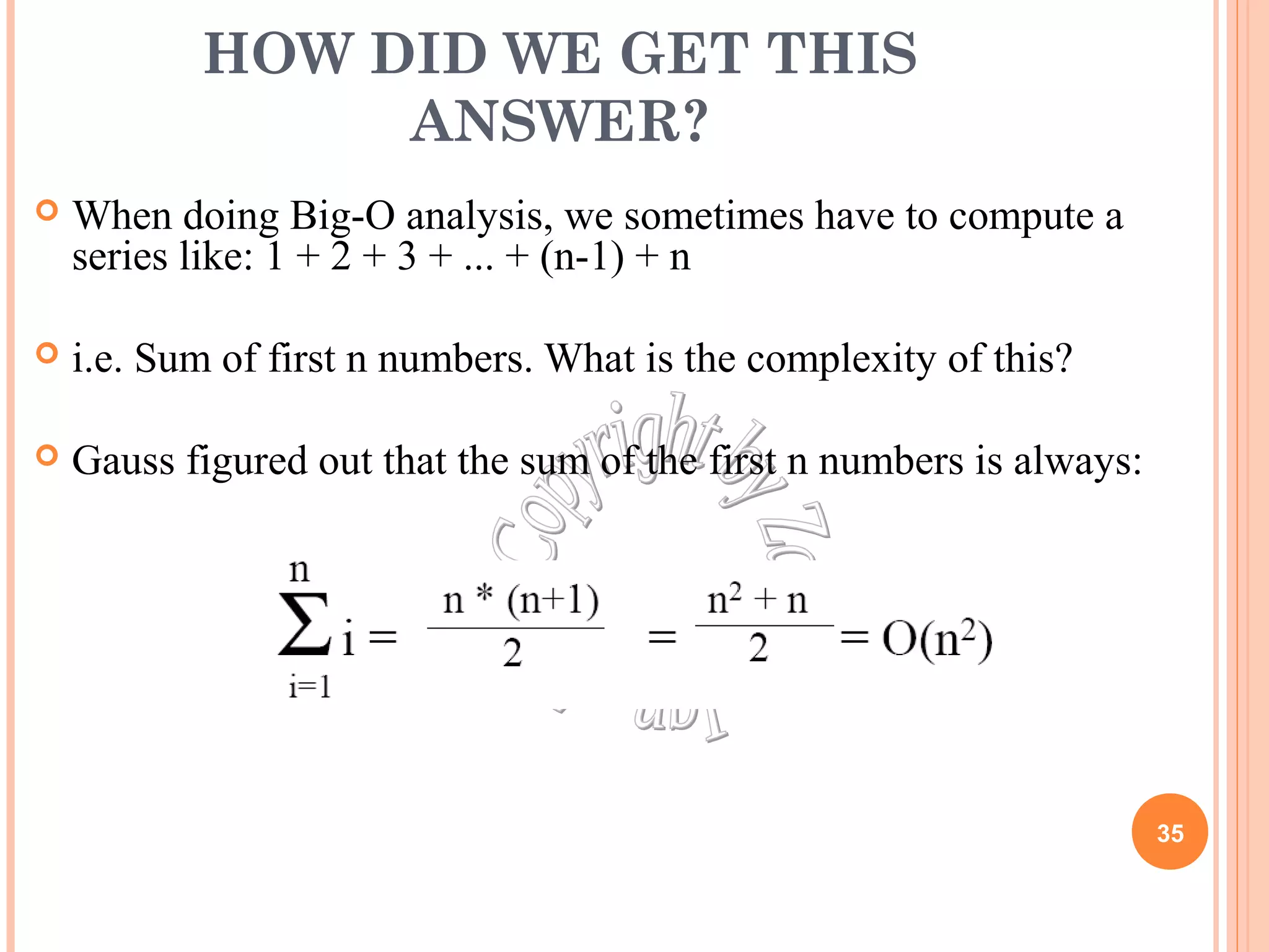
Number of iterations of the inner loop is:
0 + 1 + 2 + ... + (N-1) = O(N2)
34](https://image.slidesharecdn.com/lec03-04-timecomplexity-141021105349-conversion-gate01/75/Algorithm-And-analysis-Lecture-03-04-time-complexity-34-2048.jpg)
![ANALYZING NESTED LOOPS[3]
int K=0;
for(int i=0; i<N; i++)
{
cout <<”Hello”;
for(int j=0; j<K; j--)
Sum++;
}
36](https://image.slidesharecdn.com/lec03-04-timecomplexity-141021105349-conversion-gate01/75/Algorithm-And-analysis-Lecture-03-04-time-complexity-36-2048.jpg)
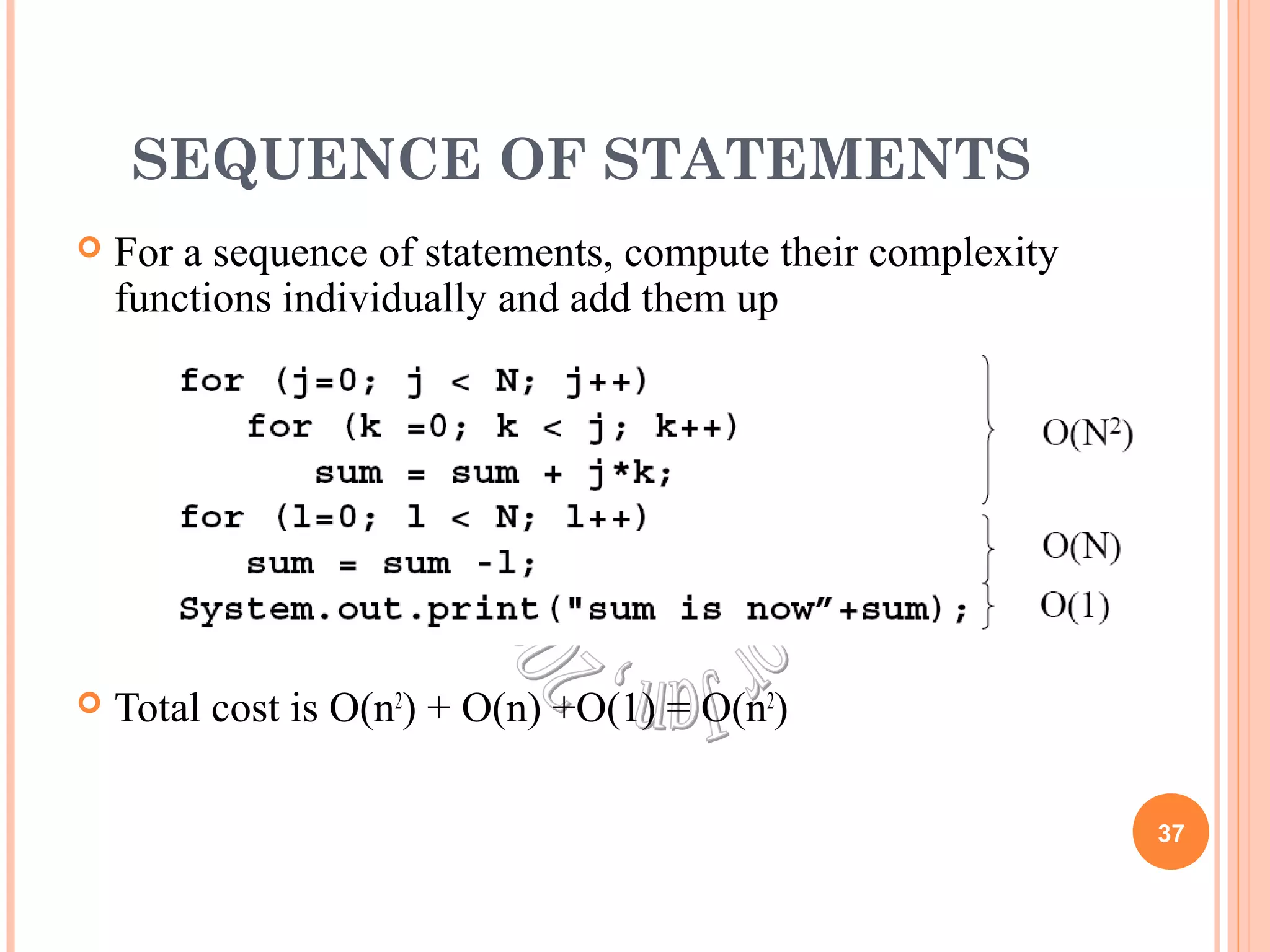
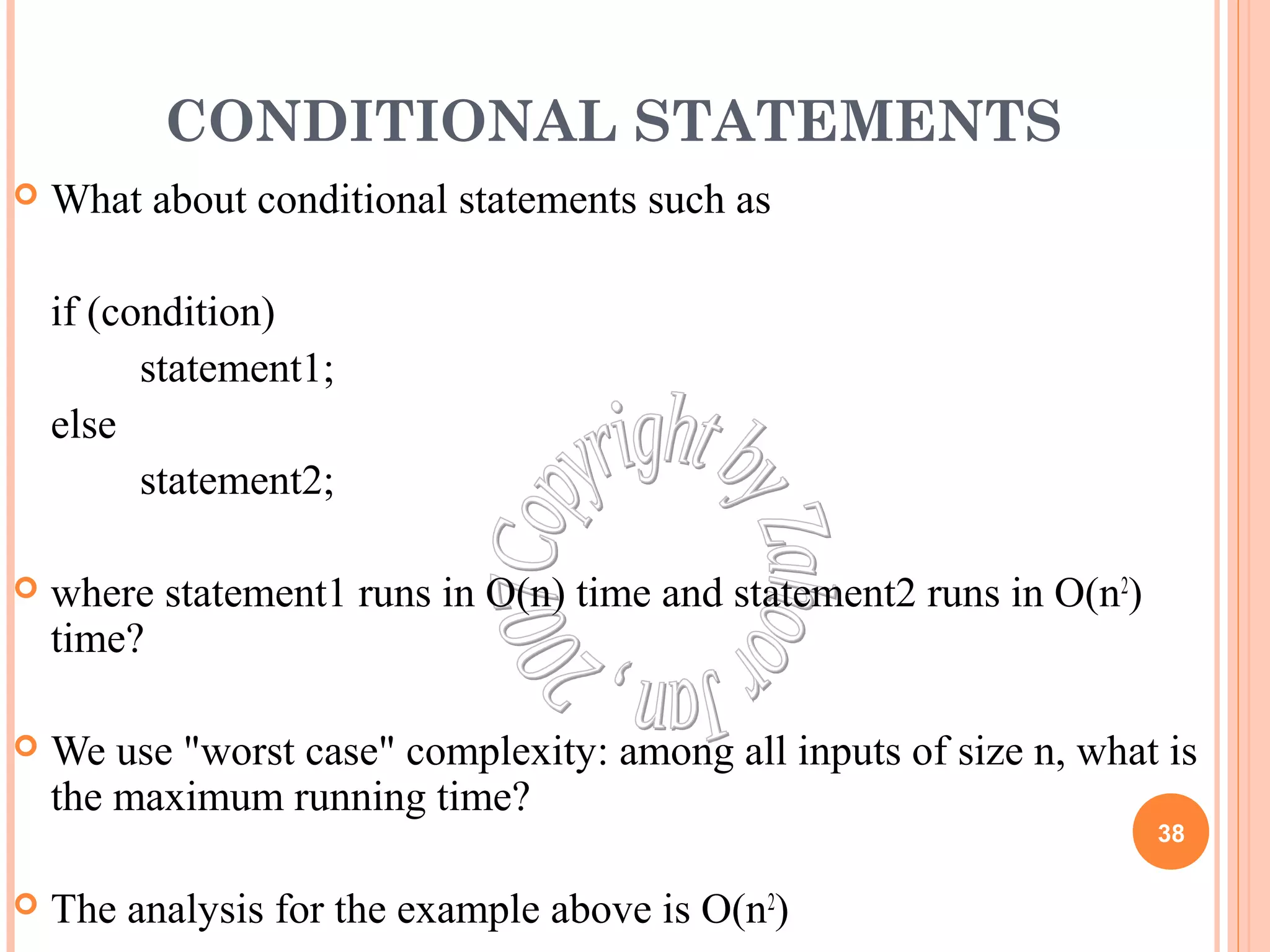
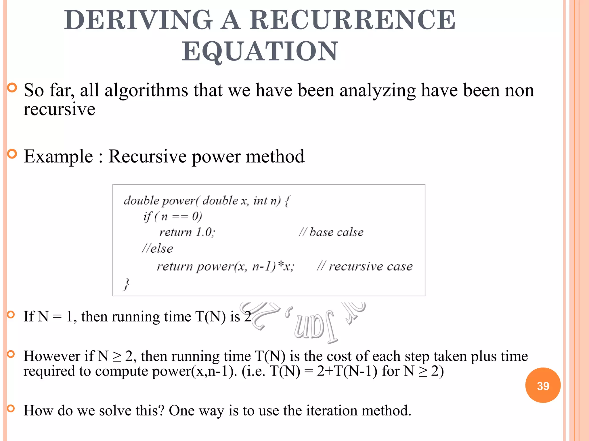
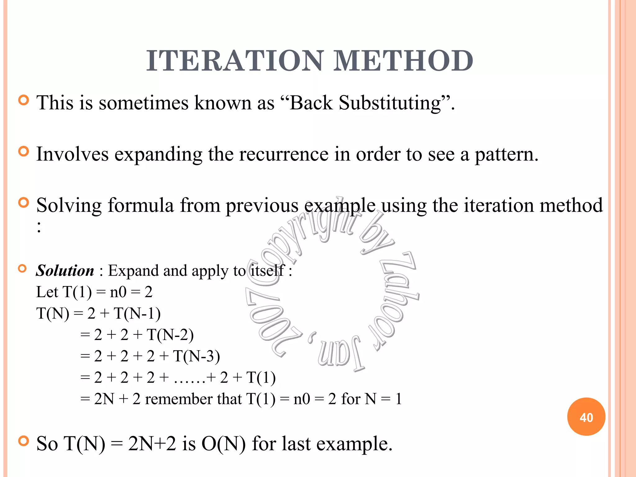

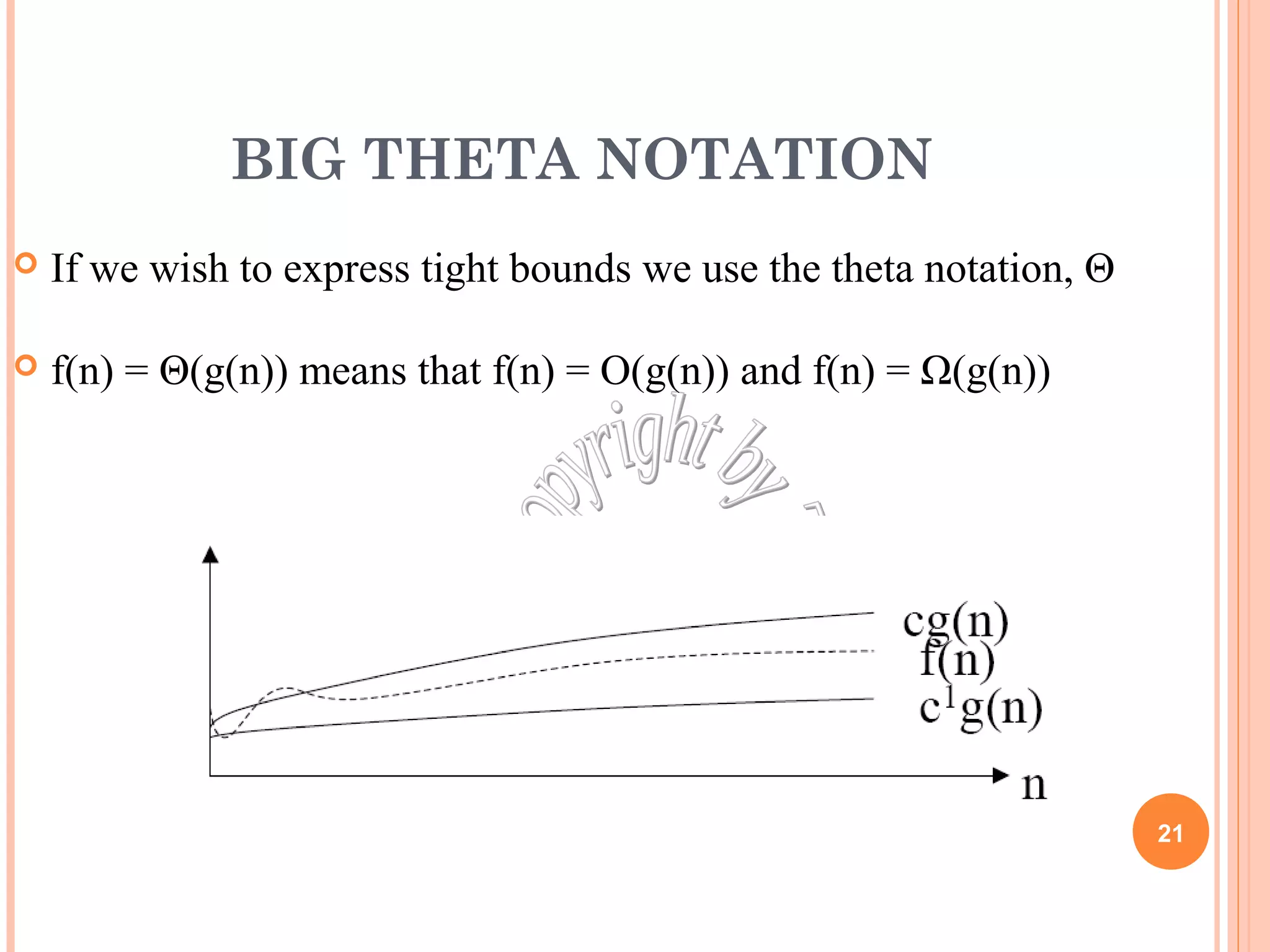
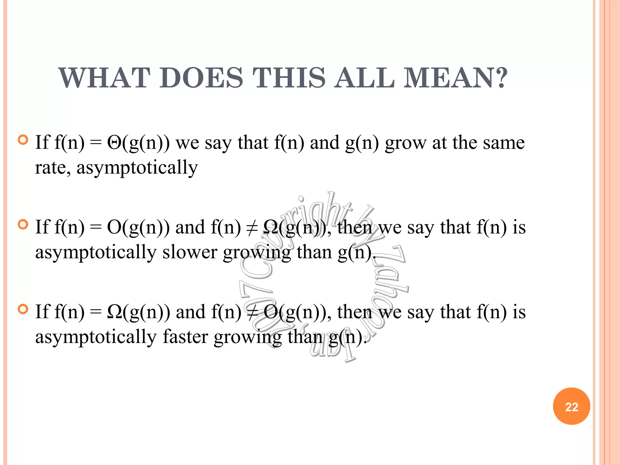
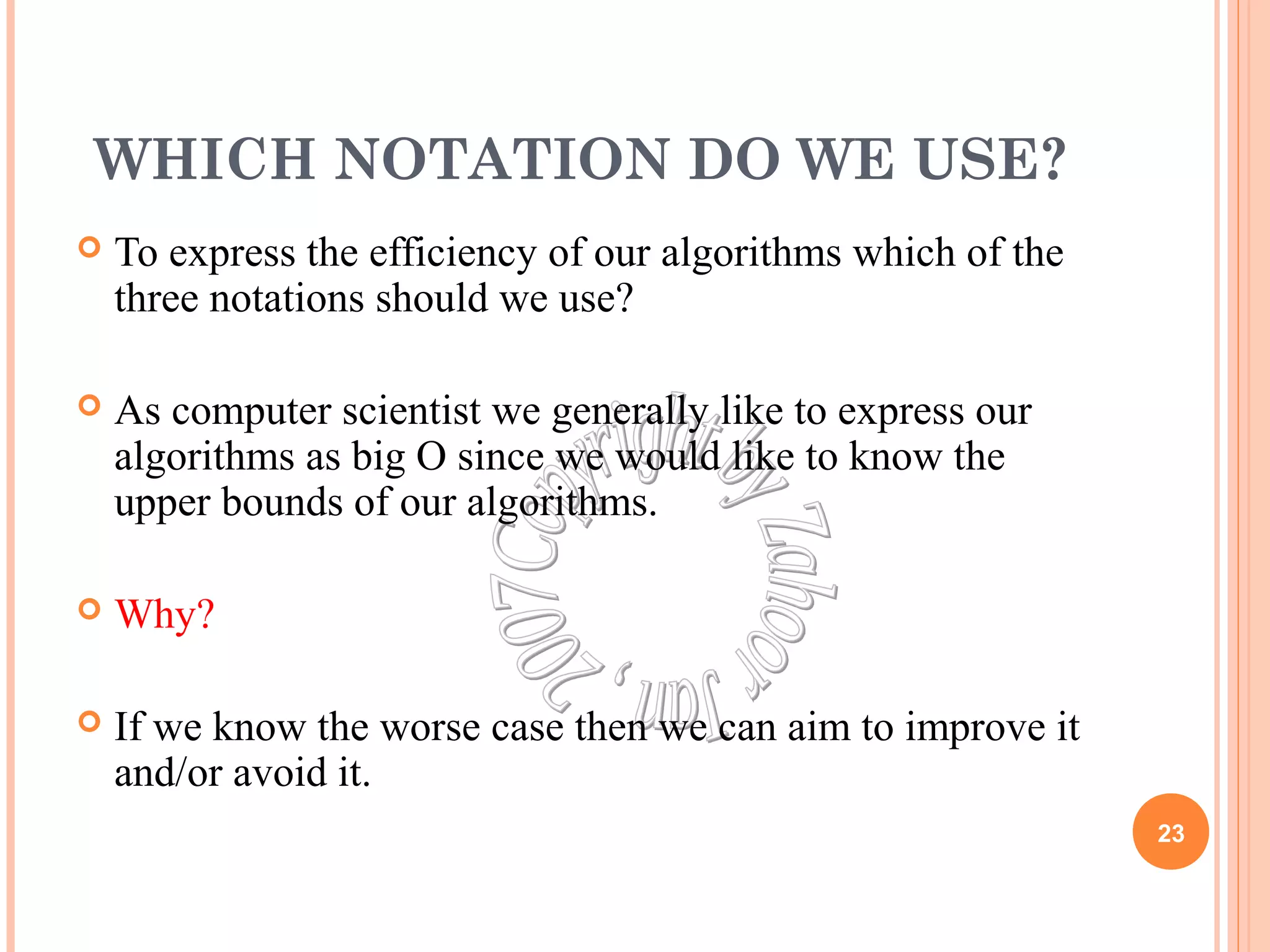
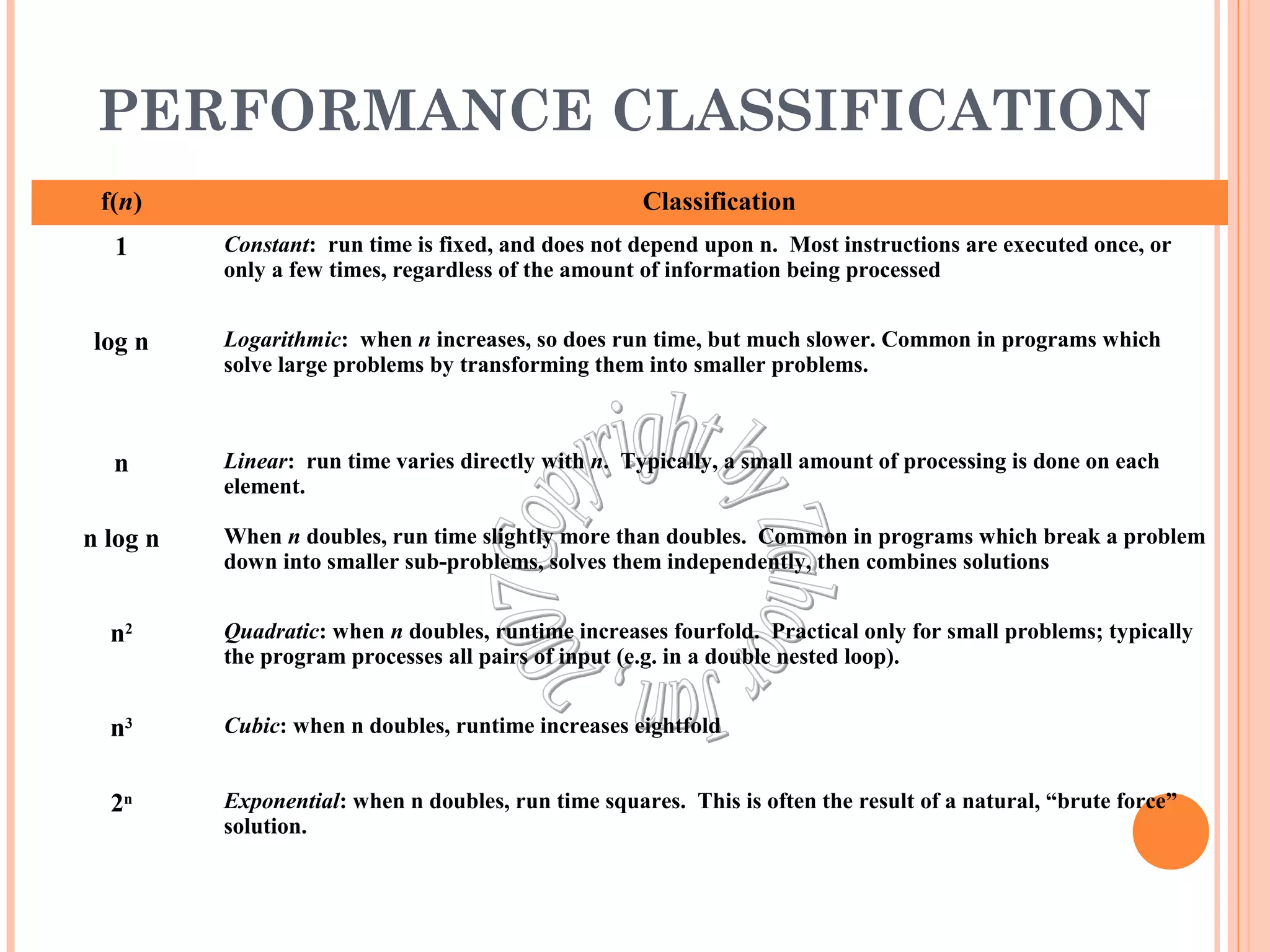
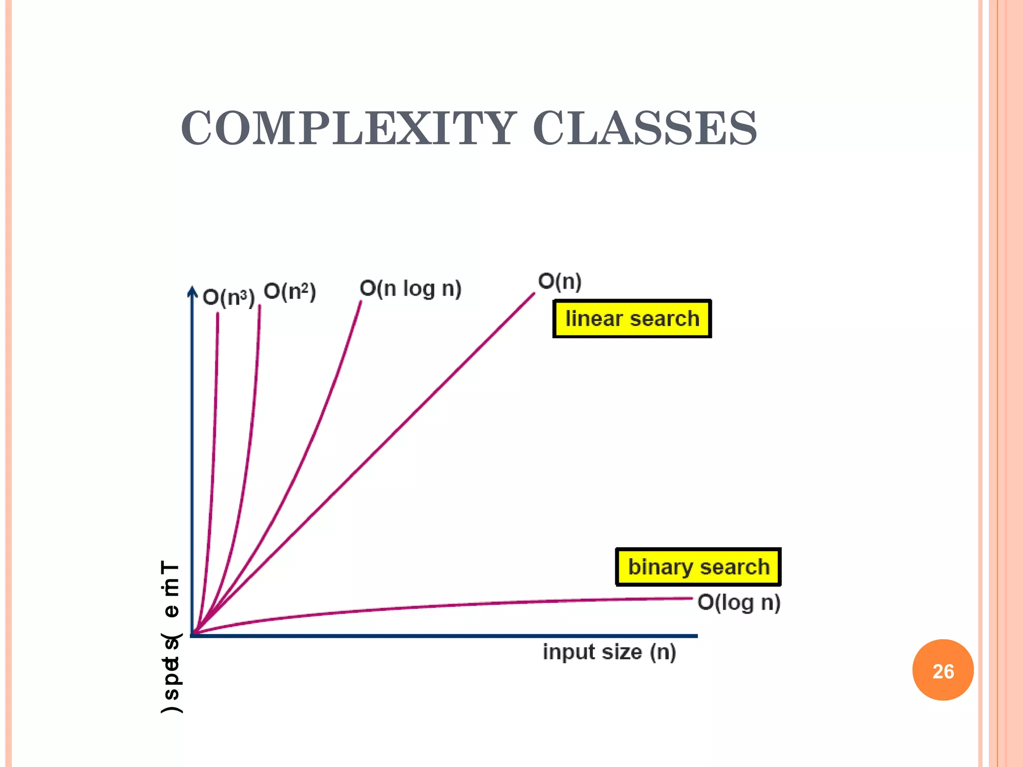
This document discusses algorithm efficiency and complexity analysis. It defines key terms like algorithms, asymptotic complexity, Big O notation, and different complexity classes. It provides examples of analyzing time complexity for different algorithms like loops, nested loops, and recursive functions. The document explains that Big O notation allows analyzing algorithms independent of machine or input by focusing on the highest order term as the problem size increases. Overall, the document introduces methods for measuring an algorithm's efficiency and analyzing its time and space complexity asymptotically.