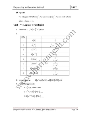
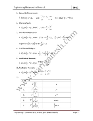
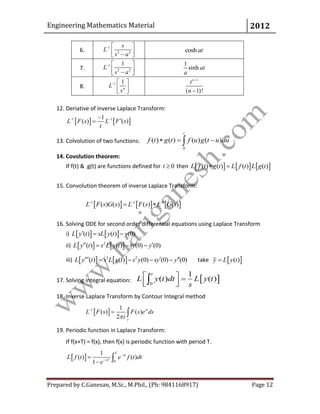
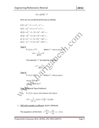
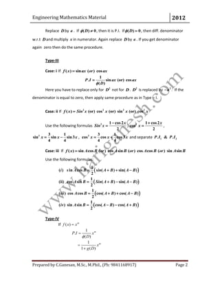
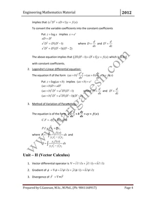
This document provides formulas and methods for solving ordinary differential equations and vector calculus problems that are covered in an Engineering Mathematics course. It includes: 1. Seven methods for finding the complementary function for ODEs with constant coefficients depending on the nature of the roots. 2. Methods for finding the particular integral for ODEs with constant coefficients, including four types of functions the right side could be. 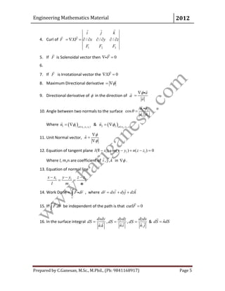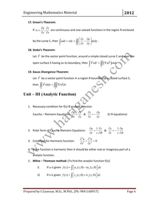3. An overview of key concepts in vector calculus including vector differential operators, gradient, divergence, curl, and theorems like Green's theorem, Stokes' theorem, and Gauss' divergence theorem.

1. Engineering Mathematics Material 2012
Prepared by C.Ganesan, M.Sc., M.Phil., (Ph: 9841168917) Page 1
SUBJECT NAME : Engineering Mathematics – II
SUBJECT CODE : MA 2161
MATERIAL NAME : Formula Material
MATERIAL CODE : JM08AM1003
Name of the Student: Branch:
Unit – I (Ordinary Differential Equation)
1. ODE with constant coefficients: Solution C.F + P.Iy 
Complementary functions:
Sl.No. Nature of Roots C.F
1. 1 2m m ( ) mx
Ax B e
2. 1 2 3m m m   2 mx
Ax Bx c e 
3. 1 2m m 1 2m x m x
Ae Be
4. 1 2 3m m m  31 2 m xm x m x
Ae Be Ce 
5. 1 2 3,m m m 3
( ) m xmx
Ax B e Ce 
6. m i   ( cos sin )x
e A x B x
 
7. m i  cos sinA x B x 
Particular Integral:
Type-I
If ( ) 0f x 
then . 0P I 
Type-II
If ( ) ax
f x e
1
.
( )
ax
P I e
D


2. Engineering Mathematics Material 2012
Prepared by C.Ganesan, M.Sc., M.Phil., (Ph: 9841168917) Page 2
Replace Dby a . If ( ) 0D  , then it is P.I. If ( ) 0D  , then diff. denominator
w.r.t Dand multiply x in numerator. Again replace Dby a . If you get denominator
again zero then do the same procedure.
Type-III
Case: i If ( ) sin ( ) cosf x ax or ax
1
. sin (or) cos
( )
P I ax ax
D

Here you have to replace only for 2
D not for D. 2
D is replaced by 2
a . If the
denominator is equal to zero, then apply same procedure as in Type – I.
Case: ii If 2 2 3 3
( ) (or) cos (or) sin (or) cosf x Sin x x x x
Use the following formulas 2 1 cos2
2
x
Sin x

 , 2 1 cos2
cos
2
x
x

 ,
x x x 3 3 1
sin sin sin3
4 4
, x x x 3 3 1
cos cos cos3
4 4
and separate 1 2. & .P I P I
Case: iii If ( ) sin cos ( ) cos sin ( ) cos cos ( ) sin sinf x A B or A B or A B or A B
Use the following formulas:
 
 
 
 
1
( ) in cos ( ) sin( )
2
1
(ii) cos sin ( ) sin( )
2
1
( ) cos cos cos( ) cos( )
2
1
( ) sin sin cos( ) cos( )
2
i s A B sin A B A B
A B Sin A B A B
iii A B A B A B
iv A B A B A B
   
   
   
   
Type-IV
If ( ) m
f x x
1
.
( )
m
P I x
D

1
1 ( )
m
x
g D



3. Engineering Mathematics Material 2012
Prepared by C.Ganesan, M.Sc., M.Phil., (Ph: 9841168917) Page 3
 
1
1 ( ) m
g D x

 
Here we can use Binomial formula as follows:
i)  
1 2 3
1 1 ...x x x x

     
ii)  
1 2 3
1 1 ...x x x x

     
iii)  
2 2 3
1 1 2 3 4 ...x x x x

     
iv)  
2 2 3
1 1 2 3 4 ...x x x x

     
v) 3 2 3
(1 ) 1 3 6 10 ...x x x x
     
vi) 3 2 3
(1 ) 1 3 6 10 ...x x x x
     
Type-V
If ( ) ax
f x e V where sin ,cos , m
V ax ax x
1
.
( )
ax
P I e V
D

First operate ax
e by replacing D by D+a.
1
( )
ax
e V
D a


Type-VI
If ( ) n
f x x V where sin ,cosV ax ax
sin I.P of
cos R.P of
iax
iax
ax e
ax e


Type-VII (Special Type Problems)
If ( ) sec (or) cosec (or) tanf x ax ax ax
1
. ( ) ( )ax ax
P I f x e e f x dx
D a

 
 
1. ODE with variable co-efficient: (Euler’s Method)
The equation is of the form
2
2
2
( )
d y dy
x x y f x
dx dx
  

4. Engineering Mathematics Material 2012
Prepared by C.Ganesan, M.Sc., M.Phil., (Ph: 9841168917) Page 4
Implies that 2 2
( 1) ( )x D xD y f x  
To convert the variable coefficients into the constant coefficients
Put logz x implies z
x e
2 2
3 3
( 1)
( 1)( 2)
xD D
x D D D
x D D D D

  
    
where
d
D
dx
 and
d
D
dz
 
The above equation implies that  ( 1) 1 ( )D D D y f x      which is O.D.E
with constant coefficients.
2. Legendre’s Linear differential equation:
The equation if of the form
2
2
2
( ) ( ) ( )
d y dy
ax b ax b y f x
dx dx
    
Put log( )z ax b  implies ( ) z
ax b e 
2 2 2
3 3 3
( )
( ) ( 1)
( ) ( 1)( 2)
ax b D aD
ax b D a D D
ax b D a D D D
 
   
     
where
d
D
dx
 and
d
D
dz
 
3. Method of Variation of Parameters:
The equation is of the form
d y dy
a b cy f x
dx dx
  
2
2
( )
1 2.C F Ay By  and
1 2.P I Py Qy 
where 2
1 2 1 2
( )y f x
P dx
y y y y
 
  and
1
1 2 1 2
( )y f x
Q dx
y y y y

 
Unit – II (Vector Calculus)
1. Vector differential operator is / / /i x j y k z         
2. Gradient of  / / /i x j y k z             
3. Divergence of F F 

5. Engineering Mathematics Material 2012
Prepared by C.Ganesan, M.Sc., M.Phil., (Ph: 9841168917) Page 5
4. Curl of F
1 2 3
/ / /
i j k
XF x y z
F F F
        
5. If F is Solenoidal vector then 0F 
6.
7. If F is Irrotational vector the 0XF 
8. Maximum Directional derivative  
9. Directional derivative of  in the direction of a
a
a


10. Angle between two normals to the surface 1 2
1 2
cos
n n
n n
 
Where   1 1 1
1 1 ( , , )at x y z
n   &   2 2 2
2 2 ( , , )at x y z
n  
11. Unit Normal vector, ˆn





12. Equation of tangent plane 1 1 1( ) ( ) ( ) 0l x x m y y n z z     
Where l, m,n are coefficient of , ,i j k in  .
13. Equation of normal line
1 1 1x x y y z z
l m n
  
 
14. Work Done =
C
F dr , where dr dxi dyj dzk  
15. If .
C
F dr be independent of the path is that curl 0F 
16. In the surface integral
ˆ.
dxdy
dS
n k
 ,
ˆ.
dydz
dS
n i
 ,
ˆ.
dzdx
dS
n j
 & ˆdS ndS

6. Engineering Mathematics Material 2012
Prepared by C.Ganesan, M.Sc., M.Phil., (Ph: 9841168917) Page 6
17. Green’s Theorem:
If , , ,
u v
u v
y x
 
 
are continuous and one-valued functions in the region R enclosed
by the curve C, then
C R
v u
udx vdy dxdy
x y
  
   
  
  .
18. Stoke’s Theorem:
Let F be the vector point function, around a simple closed curve C and over the
open surface S having as its boundary, then   ˆx
C S
F dr F nds  
19. Gauss Divergence Theorem:
Let F be a vector point function in a region R bounded by a closed surface S,
then ˆ
S V
F nds Fdv  
Unit – III (Analytic Function)
1. Necessary condition for f(z) is analytic function
Cauchy – Riemann Equations: &
u v v u
x y x y
   
  
   
(C-R equations)
2. Polar form of Cauchy-Riemann Equations:
1 1
&
u v v u
r r r r 
   
  
   
3. Condition for Harmonic function:
2 2
2 2
0
u u
x y
 
 
 
4. If the function is harmonic then it should be either real or imaginary part of a
analytic function.
5. Milne – Thomson method: (To find the analytic function f(z))
i) If u is given ( ) ( ,0) ( ,0)x yf z u z iu z dz   
ii) If v is given ( ) ( ,0) ( ,0)y xf z v z iv z dz   

7. Engineering Mathematics Material 2012
Prepared by C.Ganesan, M.Sc., M.Phil., (Ph: 9841168917) Page 7
6. To find the analytic function
i) ( ) ; ( )f z u iv if z iu v    adding these two
We have ( ) ( ) (1 ) ( )u v i u v i f z    
then ( )F z U iV  where , & ( ) (1 ) ( )U u v V u v F z i f z     
Here we can apply Milne – Thomson method for F(z).
7. Bilinear transformation:
  
  
  
  
1 2 3 1 2 3
1 2 3 1 2 3
w w w w z z z z
w w w w z z z z
   

   
Unit – IV (Complex Integration)
1. Cauchy’s Integral Theorem:
If f(z) is analytic and ( )f z is continuous inside and on a simple closed curve C,
then ( ) 0
c
f z dz  .
2. Cauchy’s Integral Formula:
If f(z) is analytic within and on a simple closed curve C and 0z is any point inside
C, then
( )
2 ( )
C
f z
dz if a
z a


3. Cauchy’s Integral Formula for derivatives:
If a function f(z) is analytic within and on a simple closed curve C and a is any
point lying in it, then
 
2
1 ( )
( )
2 C
f z
f a dz
i z a
 


Similarly
 
3
2! ( )
( )
2 C
f z
f a dz
i z a
 

 , In general
 
( )
1
! ( )
( )
2
n
n
C
n f z
f a dz
i z a 



4. Cauchy’s Residue theorem:
If f(z) be analytic at all points inside and on a simple closed cuve c, except for a
finite number of isolated singularities 1 2 3, , ,... nz z z z inside c, then
( ) 2 (sum of the residues of ( ))
C
f z dz i f z .

8. Engineering Mathematics Material 2012
Prepared by C.Ganesan, M.Sc., M.Phil., (Ph: 9841168917) Page 8
5. Critical point:
The point, at which the mapping w = f(z) is not conformal, (i.e) ( ) 0f z  is called
a critical point of the mapping.
6. Fixed points (or) Invariant points:
The fixed points of the transformation
az b
w
cz d



is obtained by putting w = z in
the above transformation, the point z = a is called fixed point.
7. Re { ( )} ( ) ( )
z a
s f z Lt z a f z

  (Simple pole)
8.   
1
1
1
Re { ( )} ( )
( 1)!
m
m
mz a
d
s f z Lt z a f z
m dz


 

(Multi Pole (or) Pole of order m)
9.
( )
Re { ( )}
( )z a
P z
s f z Lt
Q z


10. Taylor Series:
A function ( )f z , analytic inside a circle C with centre at a, can be expanded in
the series
2 3
( )( ) ( ) ( ) ( )
( ) ( ) ( ) ( ) ( ) ... ( ) ...
1! 2! 3! !
n
nz a z a z a z a
f z f a f a f a f a f a
n
   
        
Maclaurin’s Series:
Taking a = 0, Taylor’s series reduce to
2 3
( ) (0) (0) (0) (0) ...
1! 2! 3!
z z z
f z f f f f      
11. Laurent’s Series:
0 1
( ) ( )
( )
n n
n n
n n
b
f z a z a
z a
 
 
  

 
where
1
1
1 ( )
2 ( )
n n
C
f z
a dz
i z a 

 &
2
1
1 ( )
2 ( )
n n
C
f z
b dz
i z a 

 , the integrals being
taken anticlockwise.
12. Isolated Singularity:
A point 0z z is said to be isolated singularity of ( )f z if ( )f z is not analytic at
0z z and there exists a neighborhood of 0z z containing no other singularity.

9. Engineering Mathematics Material 2012
Prepared by C.Ganesan, M.Sc., M.Phil., (Ph: 9841168917) Page 9
Example:
1
( )f z
z
 . This function is analytic everywhere except at 0z  .
0z  is an isolated singularity.
13. Removable Singularity:
A singular point 0z z is called a removable singularity of ( )f z if
0
lim ( )f z
z z
exists finitely.
Example:
sin
lim ( ) lim 1
0 0
z
f z
z
z z
 
 
(finite) 0z  is a removable
singularity.
14. Essential Singularity:
If the principal part contains an infinite number of non zero terms, then 0z z is
known as a essential singularity.
Example:
 
21
1/1/
( ) 1 ...
1! 2!
z
zz
f z e     has 0z  as an essential
singularity.
CONTOUR INTEGRATION:
15. Type: I
The integrals of the form
2
0
(cos ,sin )f d

   Here we shall choose the contour
as the unit circle : 1 or ,0 2i
C z z e
     . On this type
2
1
cos
2
z
z


 ,
2
1
sin
2
z
iz


 and
1
d dz
iz
  .
16. Type: II
Improper integrals of the form
( )
( )
P x
dx
Q x


 , where P(x) and Q(x) are polynomials
in x such that the degree of Q exceeds that of P at least by two and Q(x) does not
vanish for any x. Here ( ) ( ) ( )
R
C R
f z dz f x dx f z dz


    as ( ) 0R f z dz

   .

10. Engineering Mathematics Material 2012
Prepared by C.Ganesan, M.Sc., M.Phil., (Ph: 9841168917) Page 10
17. Type: III
The integrals of the form ( )cos (or) ( )sinf x mxdx f x mxdx
 
   where
( ) 0 asf x x   .
Unit – V (Laplace Transform)
1. Definition:   0
( ) ( )st
L f t e f t dt


 
2.
Sl.No
1.  1L
1
s
2.
n
L t   1 1
! ( 1)
n n
n n
s s 
 

3.
at
L e  
1
s a
4.
at
L e
  
1
s a
5.  sinL at 2 2
a
s a
6.  cosL at 2 2
s
s a
7.  sinhL at 2 2
a
s a
8.  coshL at 2 2
s
s a
3. Linear Property:      ( ) ( ) ( ) ( )L af t bg t aL f t bL g t  
4. First Shifting property:
If  ( ) ( )L f t F s , then
i)  ( ) ( )at
s s a
L e f t F s  
   
ii)  ( ) ( )at
s s a
L e f t F s
 
   

11. Engineering Mathematics Material 2012
Prepared by C.Ganesan, M.Sc., M.Phil., (Ph: 9841168917) Page 11
5. Second Shifting property:
If  ( ) ( )L f t F s ,
( ),
( )
0,
f t a t a
g t
t a
 
 

then  ( ) ( )as
L g t e F s

6. Change of scale:
If  ( ) ( )L f t F s , then  
1
( )
s
L f at F
a a
 
  
 
7. Transform of derivative:
If  ( ) ( )L f t F s , then  ( ) ( )
d
L tf t F s
ds
  ,
2
2
2
( ) ( )
d
L t f t F s
ds
    ,
In general ( ) ( 1) ( )
n
n n
n
d
L t f t F s
ds
    
8. Transform of Integral;
If  ( ) ( )L f t F s , then
1
( ) ( )
s
L f t F s ds
t

 
  

9. Initial value Theorem:
If  ( ) ( )L f t F s , then
( ) ( )
0 s
Lt f t Lt sF s
t

  
10. Final value Theorem:
If  ( ) ( )L f t F s , then
( ) ( )
s 0
Lt f t Lt sF s
t

  
11.
Sl.No
1.
1 1
L
s
  
  
1
2.
1 1
L
s a
  
  
at
e
3.
1 1
L
s a
  
  
at
e
4.
1
2 2
s
L
s a
  
  
cosat
5.
1
2 2
1
L
s a
  
  
1
sin at
a

12. Engineering Mathematics Material 2012
Prepared by C.Ganesan, M.Sc., M.Phil., (Ph: 9841168917) Page 12
6.
1
2 2
s
L
s a
  
  
coshat
7.
1
2 2
1
L
s a
  
  
1
sinh at
a
8.
1 1
n
L
s
  
  
1
( 1)!
n
t
n


12. Deriative of inverse Laplace Transform:
   1 11
( ) ( )L F s L F s
t
 

13. Colvolution of two functions:
0
( ) ( ) ( ) ( )
t
f t g t f u g t u du  
14. Covolution theorem:
If f(t) & g(t) are functions defined for 0t  then      ( ) ( ) ( ) ( )L f t g t L f t L g t 
15. Convolution theorem of inverse Laplace Transform:
     1 1 1
( ) ( ) ( ) ( )L F s G s L F s L G s  
 
16. Solving ODE for second order differential equations using Laplace Transform
i)    ( ) ( ) (0)L y t sL y t y  
ii)    2
( ) ( ) (0) (0)L y t s L y t sy y   
iii)    3 2
( ) ( ) (0) (0) (0)L y t s L y t s y sy y      take  ( )y L y t
17. Solving integral equation:  0
1
( ) ( )
t
L y t dt L y t
s
  
  
18. Inverse Laplace Transform by Contour Integral method
 1 1
( ) ( )
2
st
c
L F s F s e ds
i

 
19. Periodic function in Laplace Transform:
If f(x+T) = f(x), then f(x) is periodic function with period T.
  0
1
( ) ( )
1
T
st
sT
L f t e f t dt
e



 