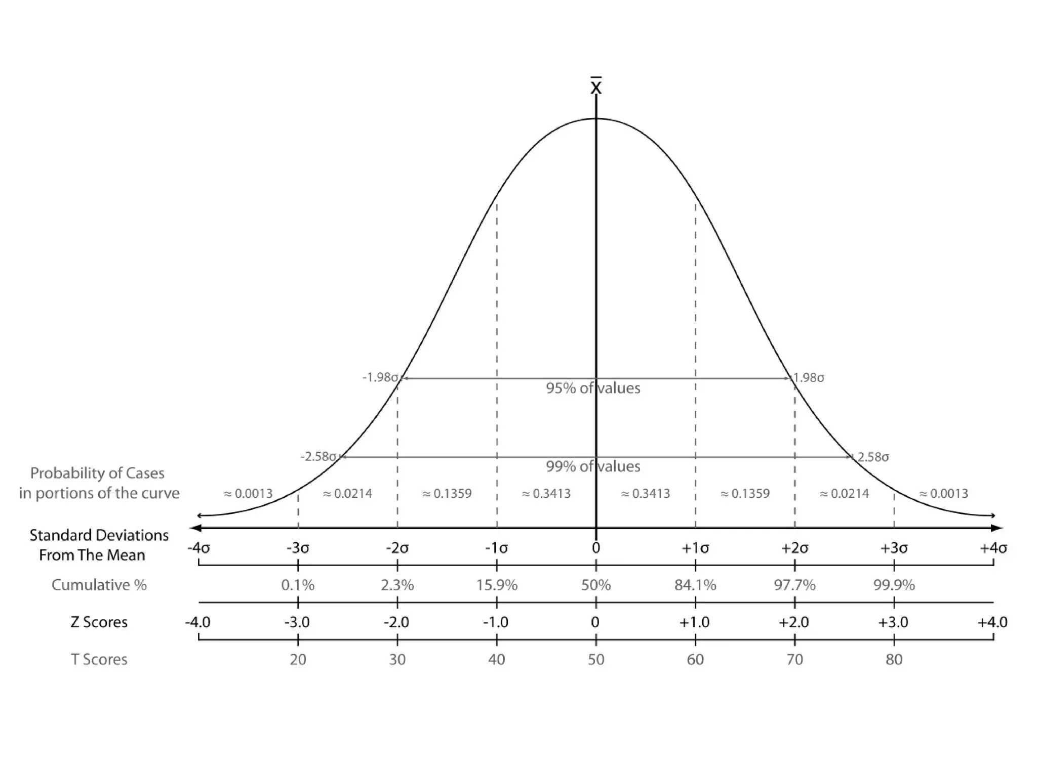
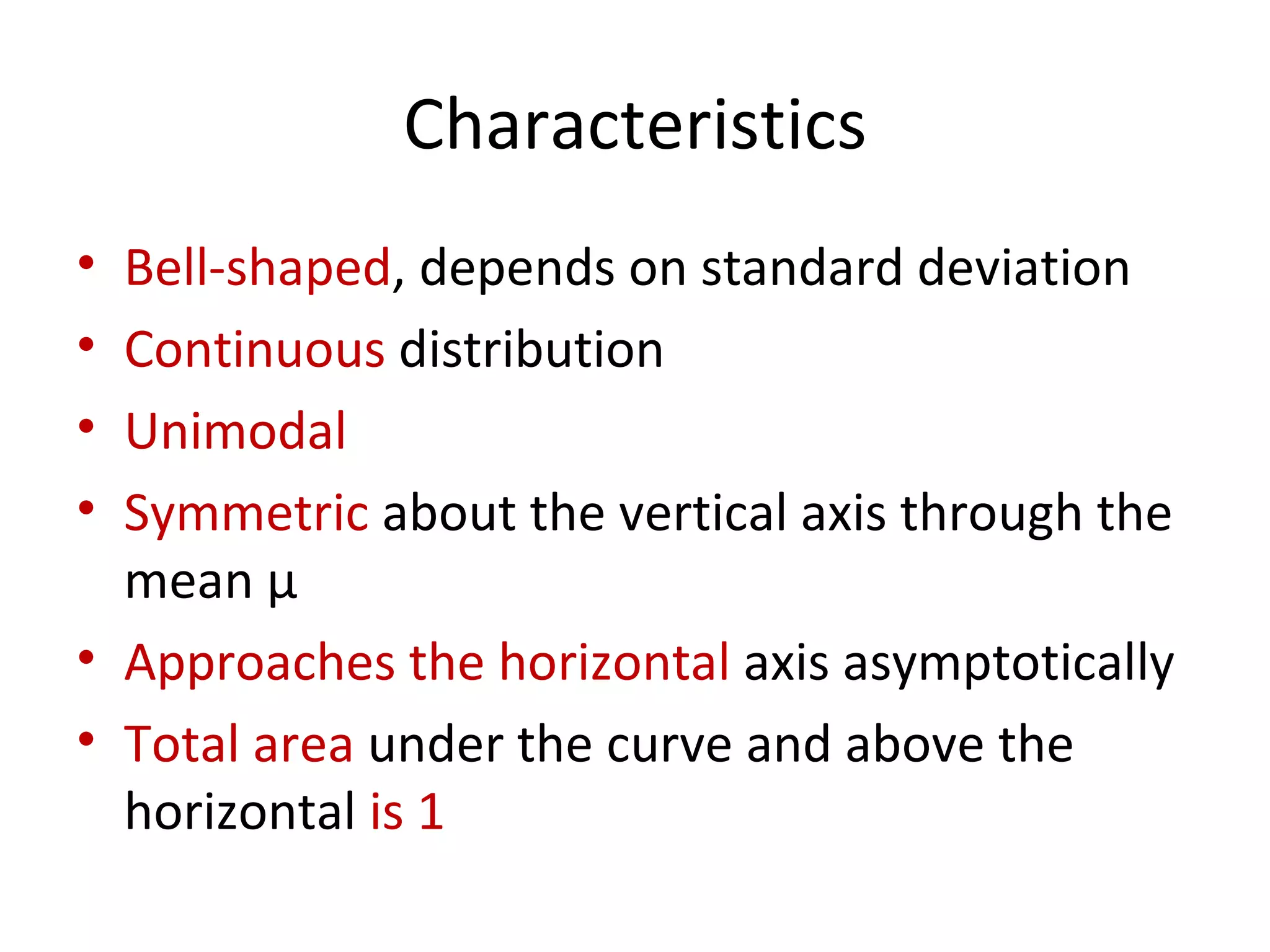
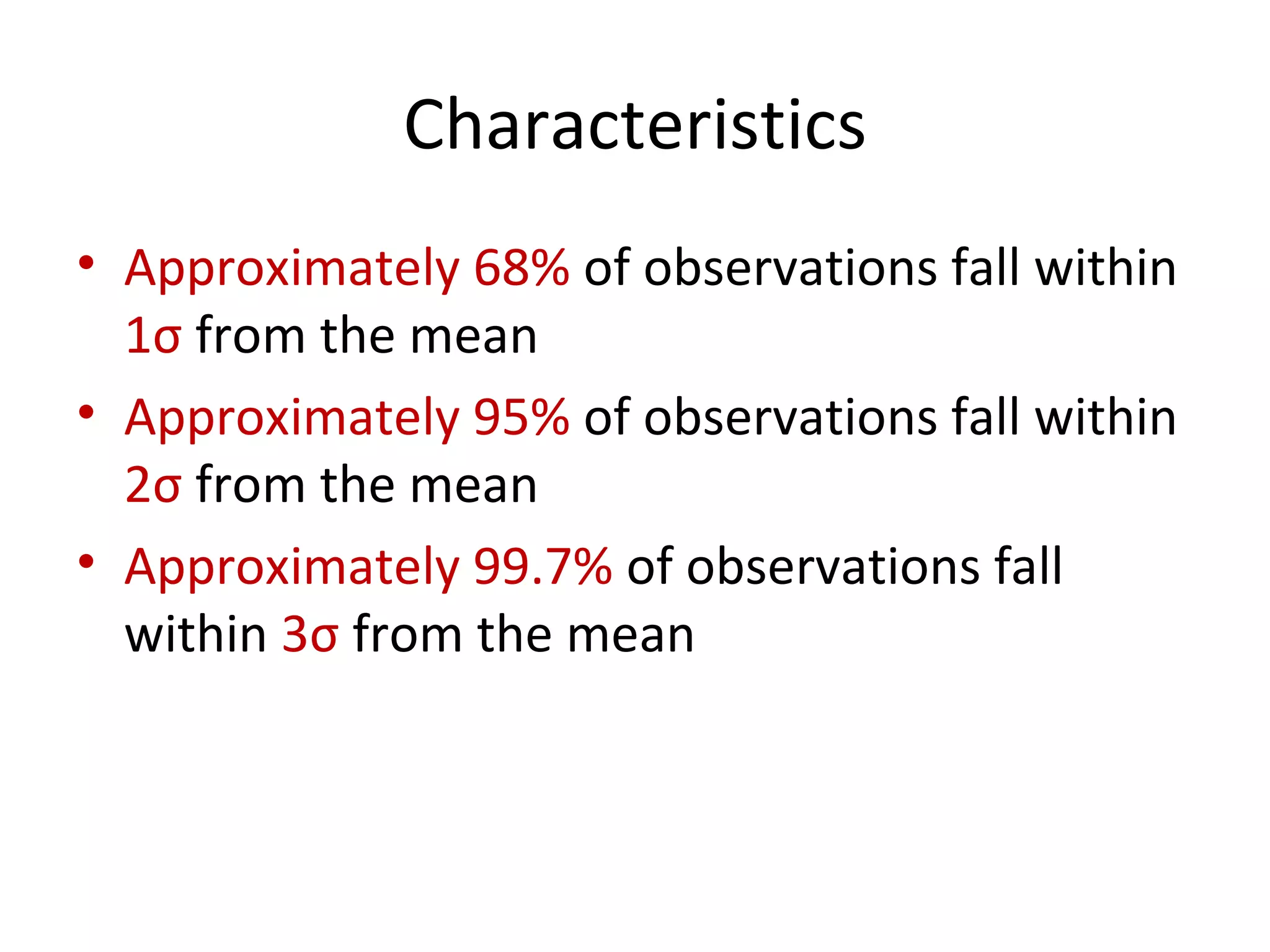
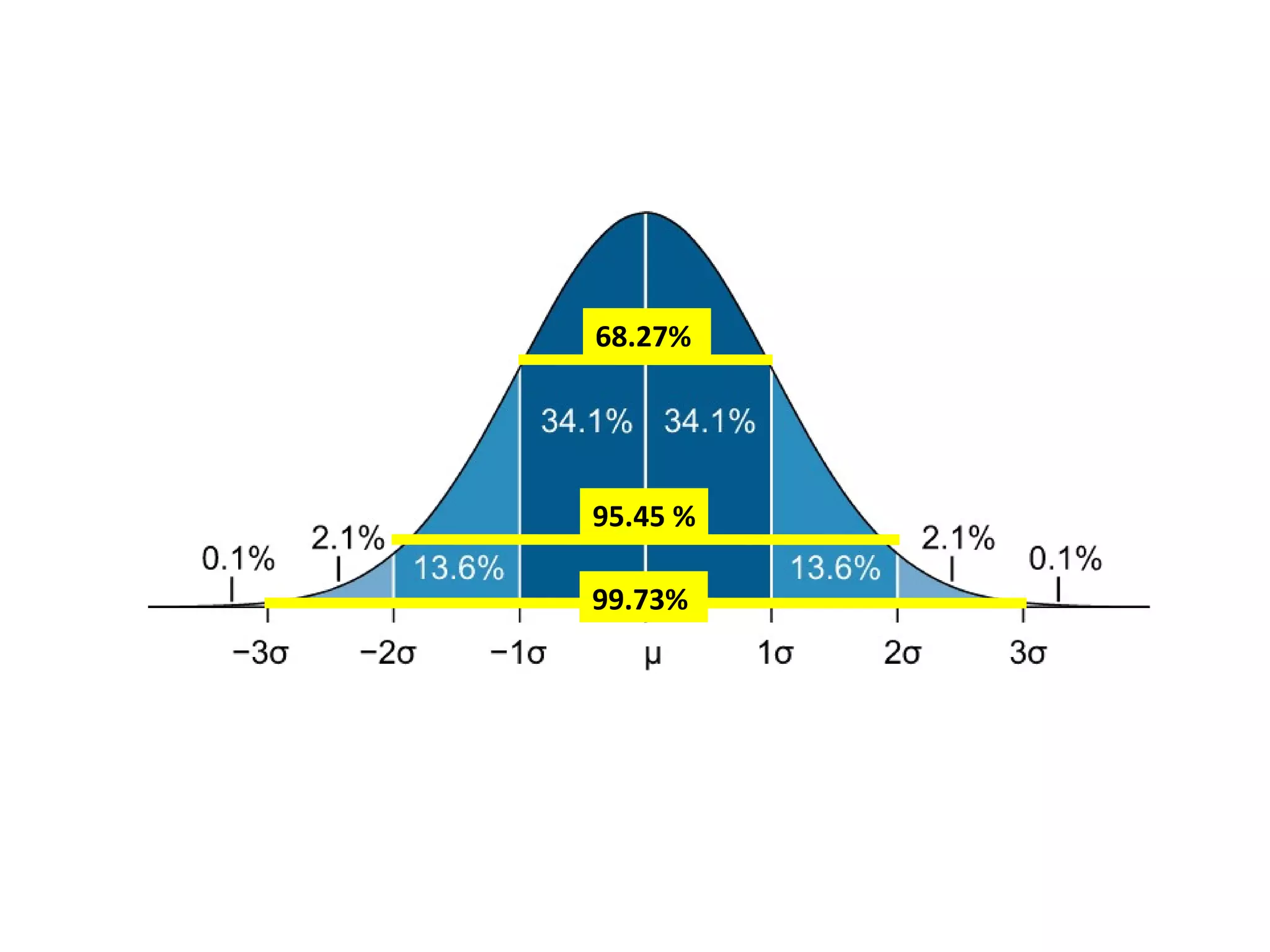
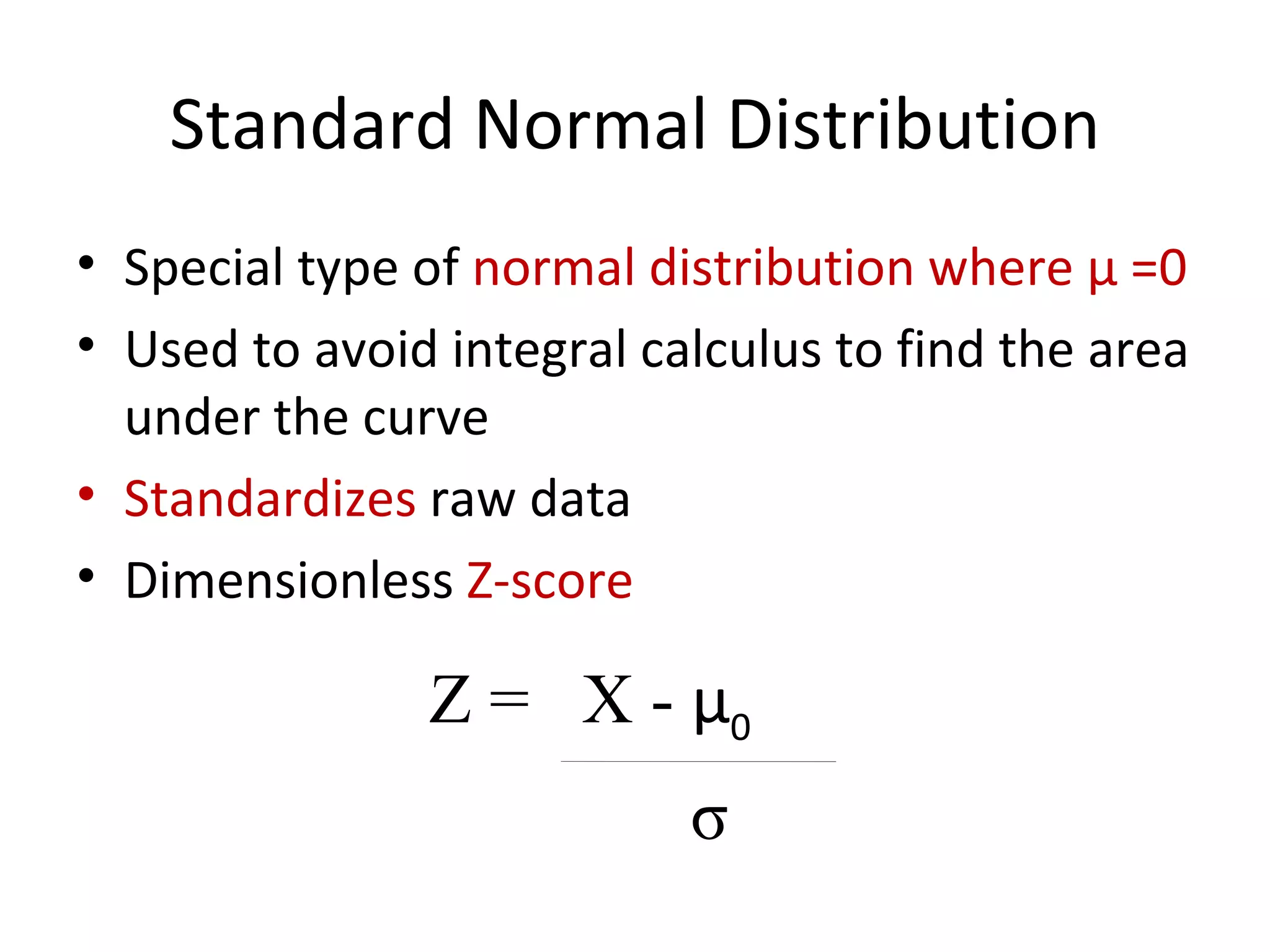
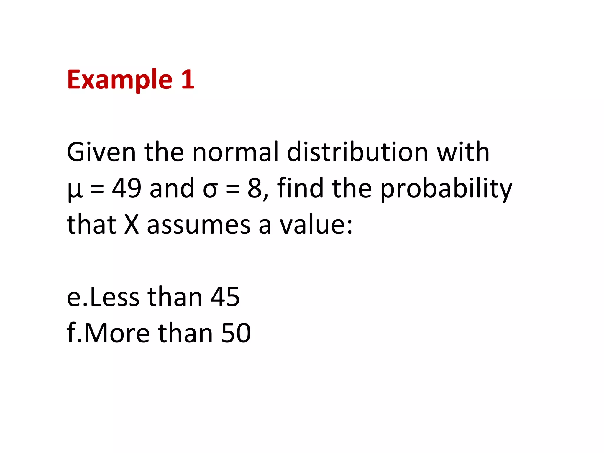
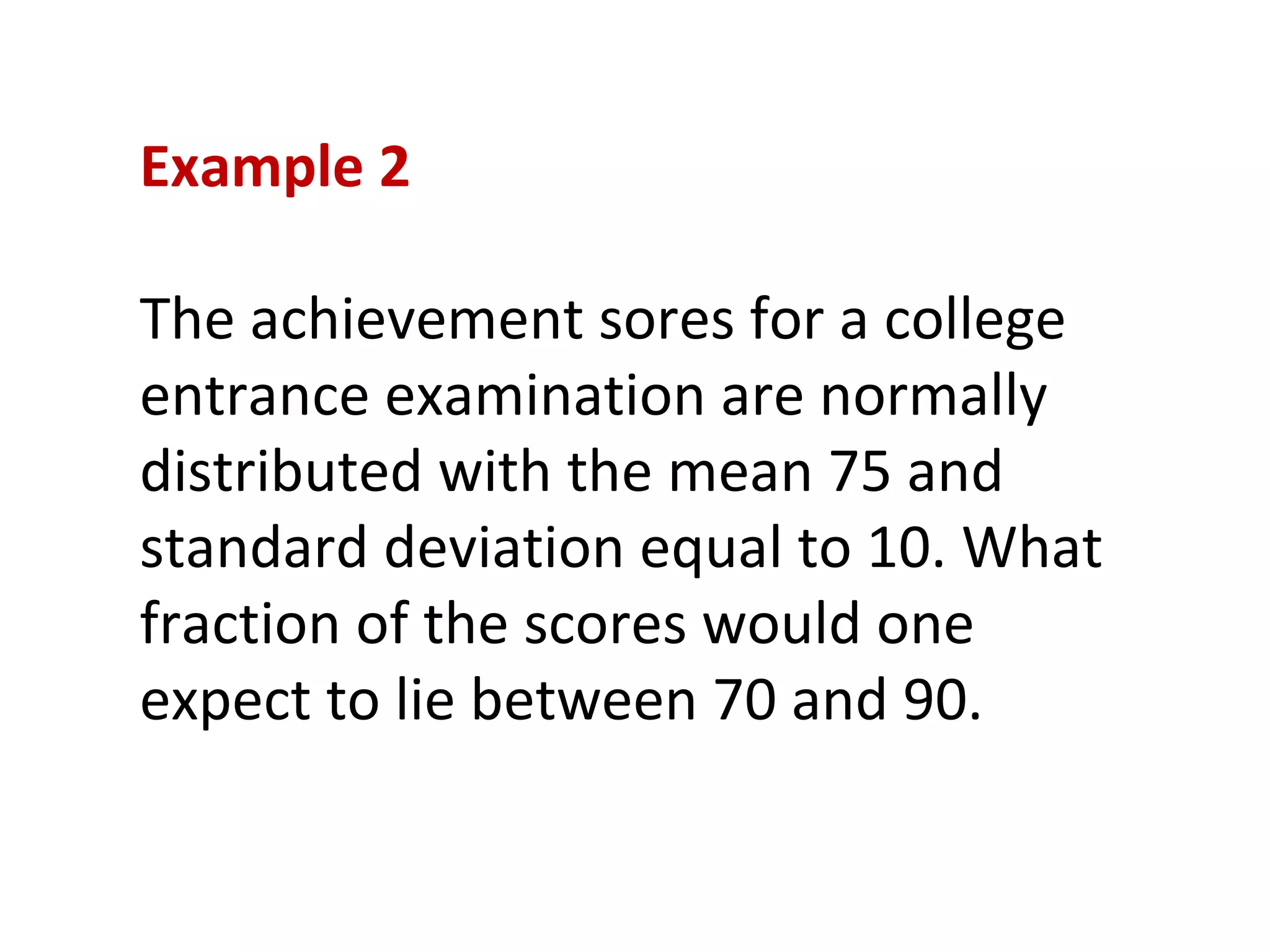
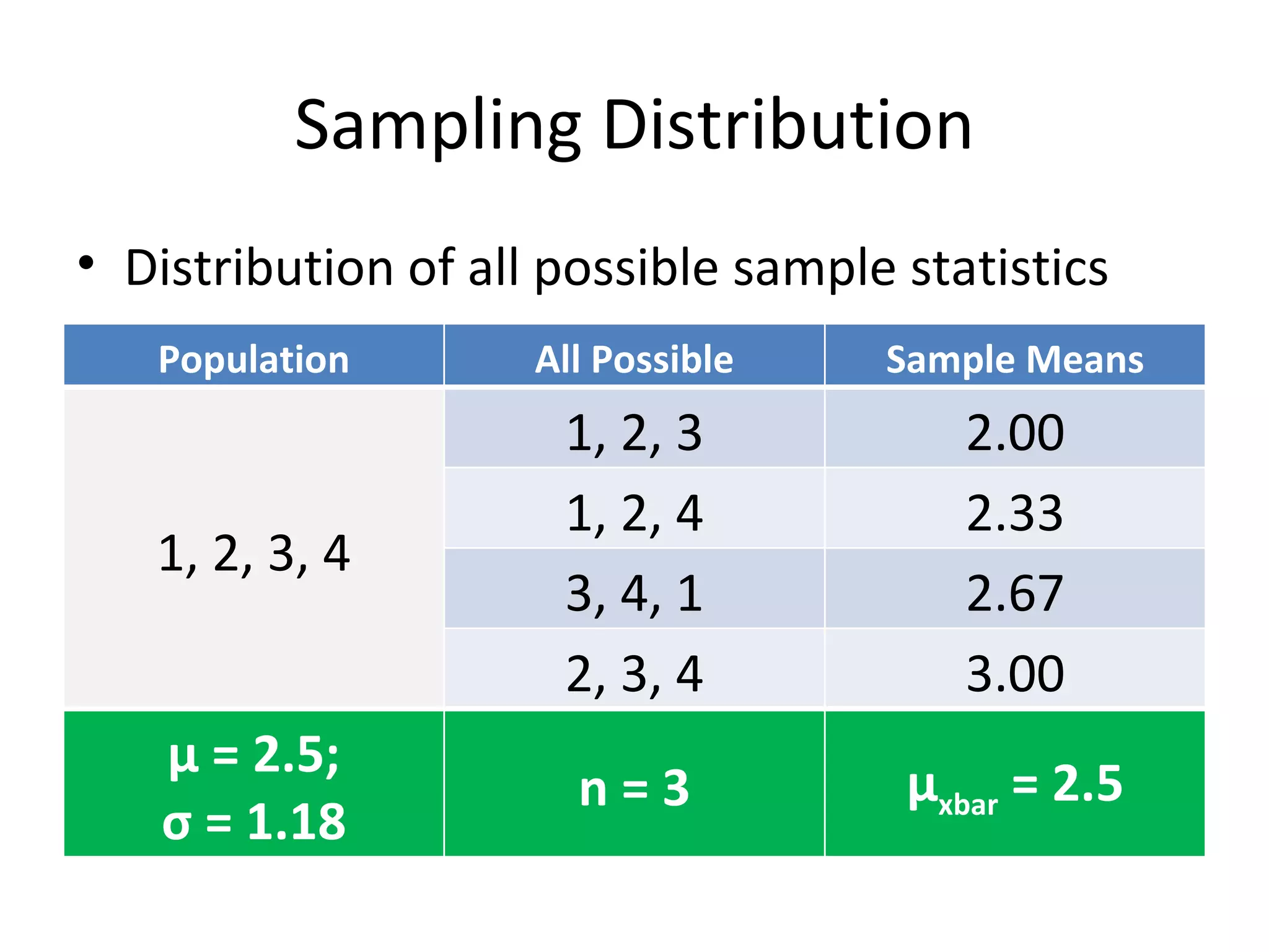
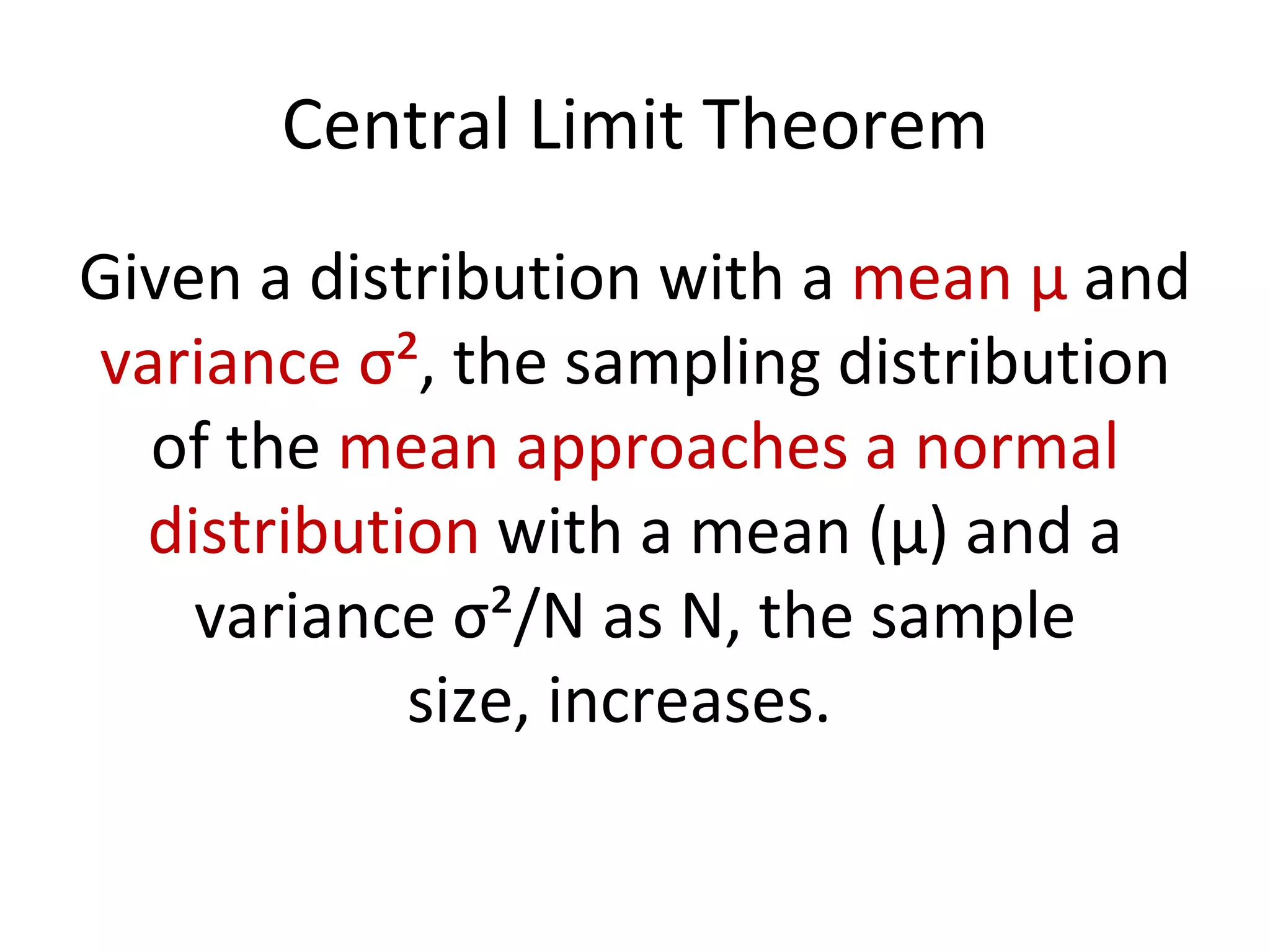
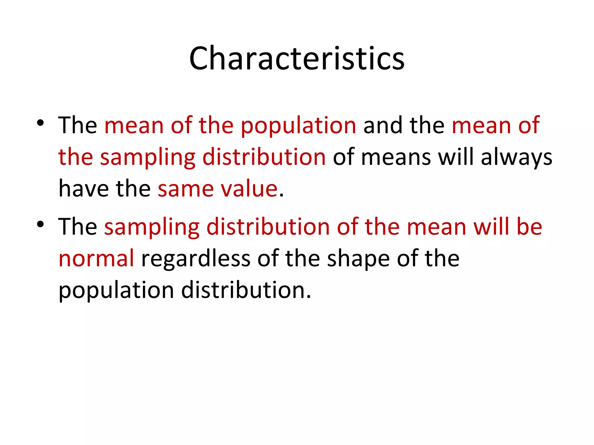
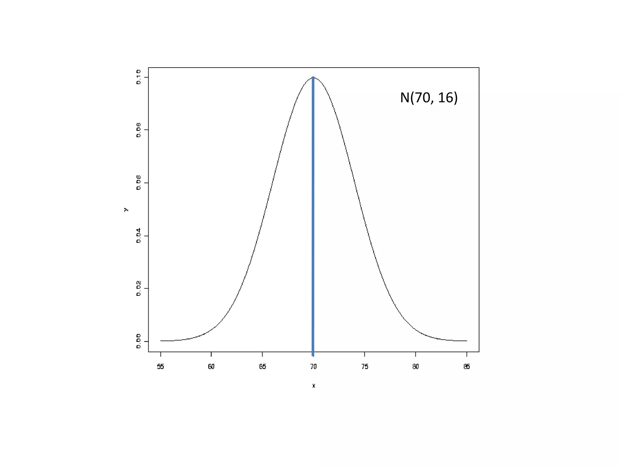
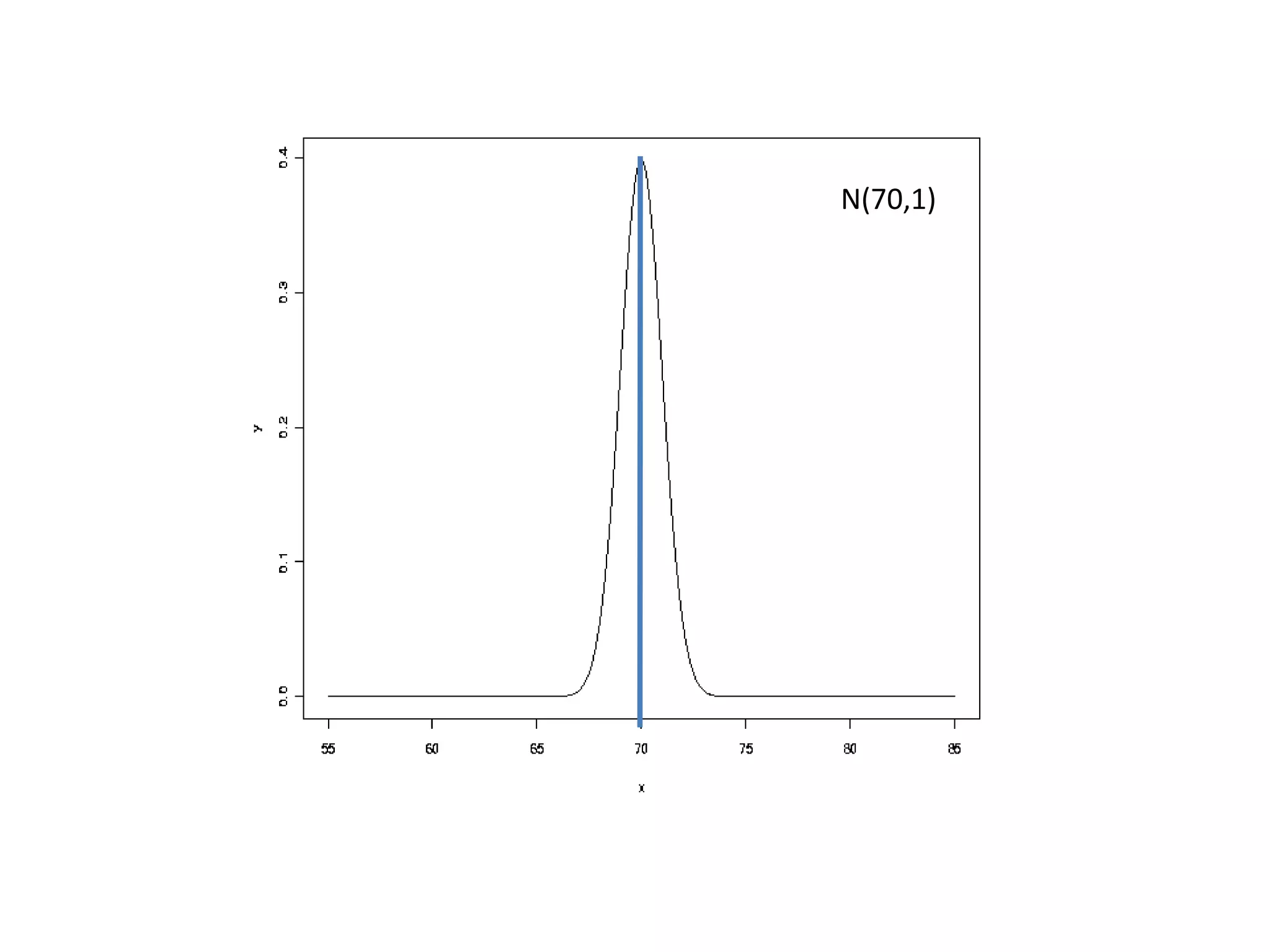
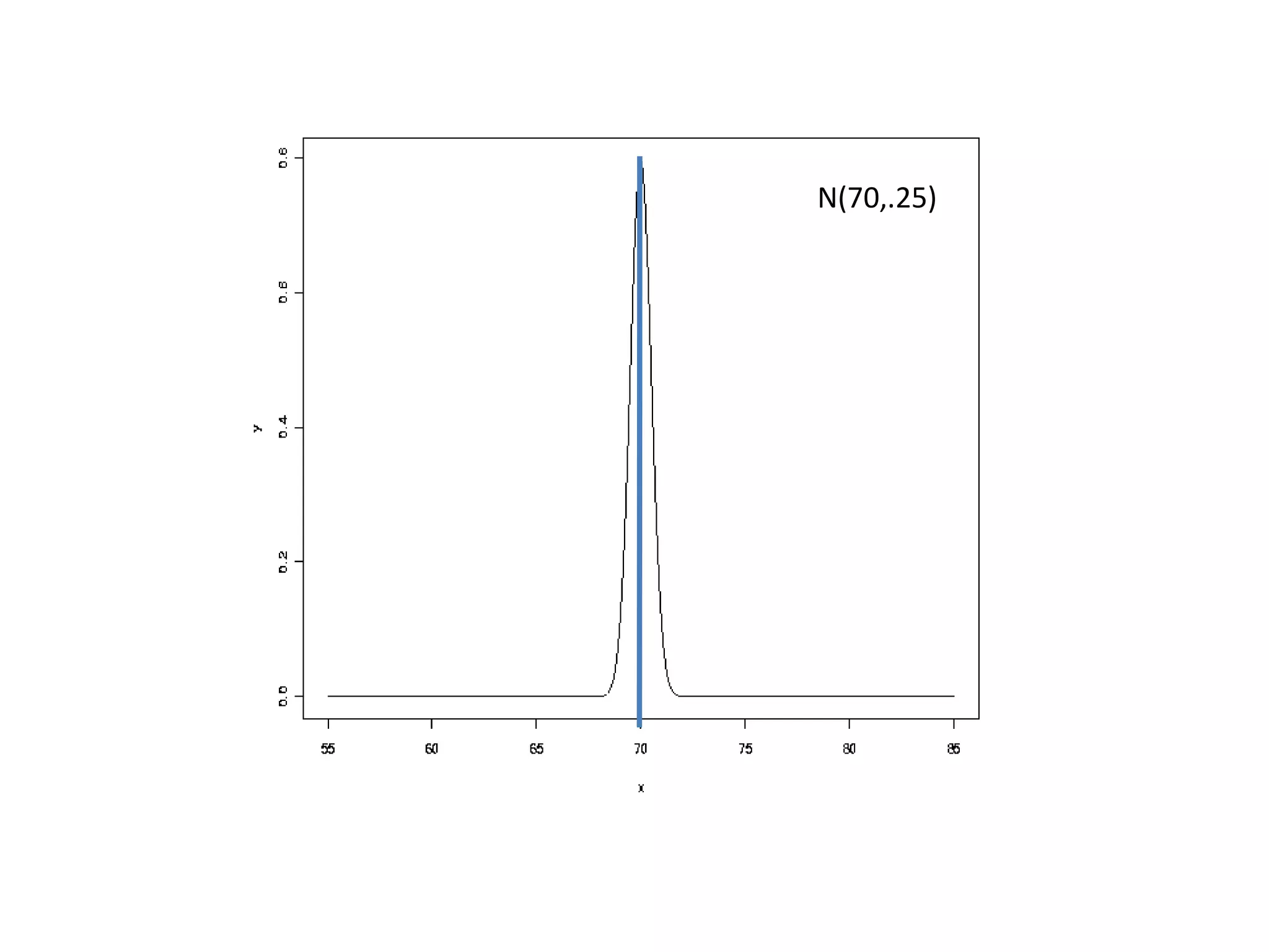
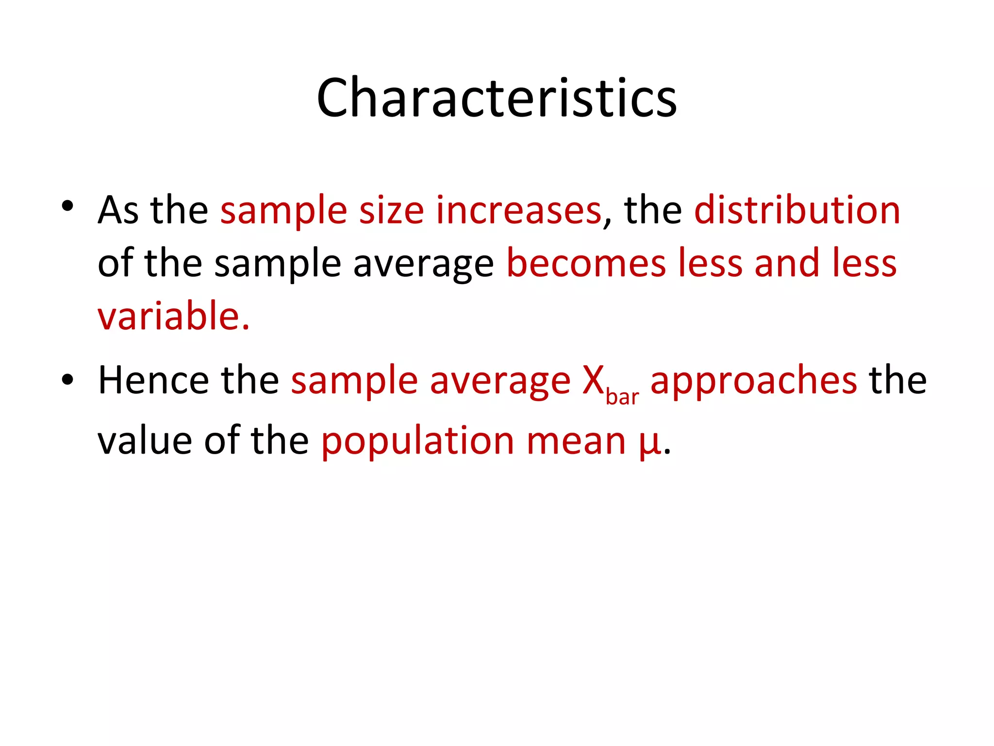
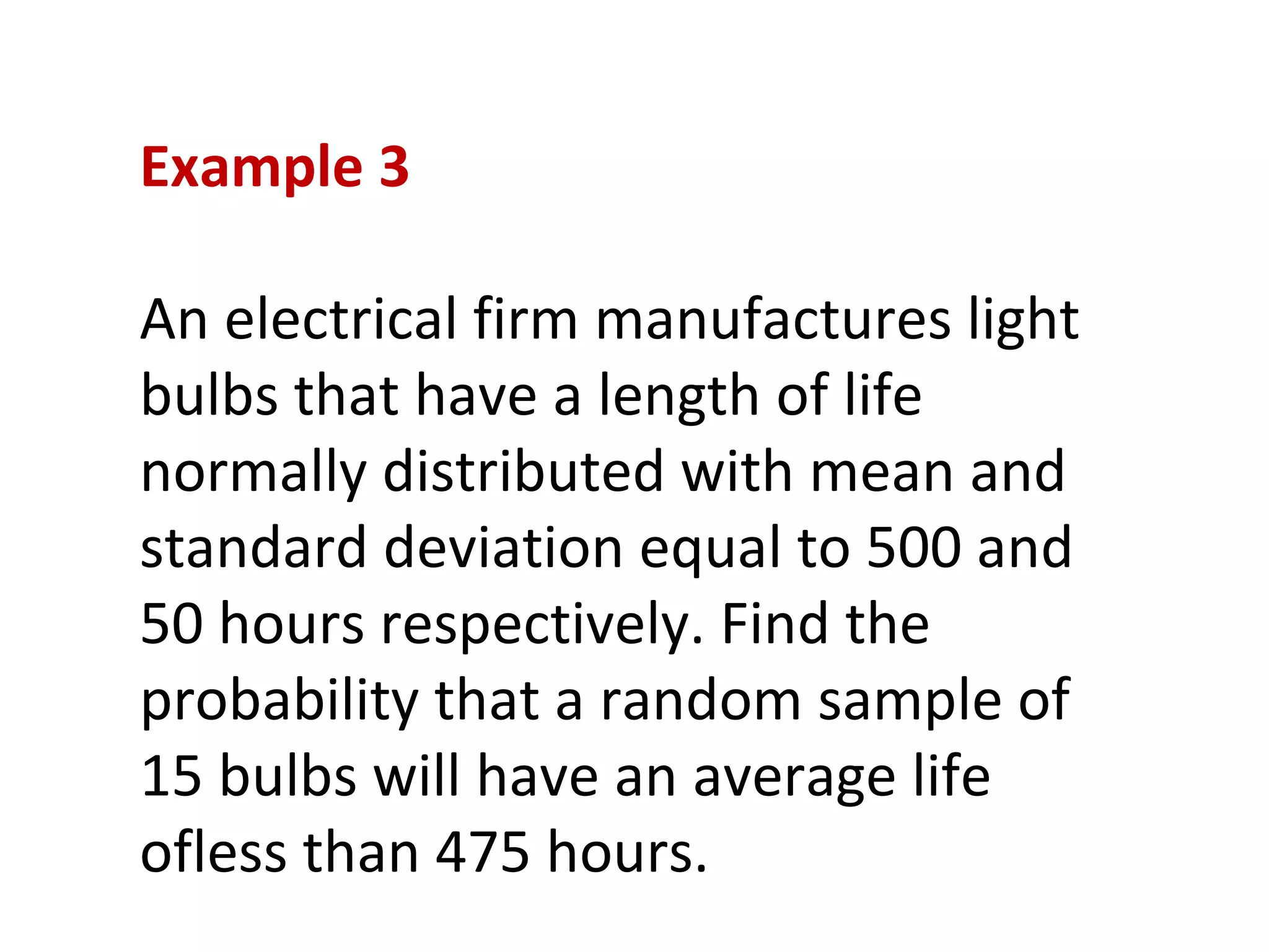
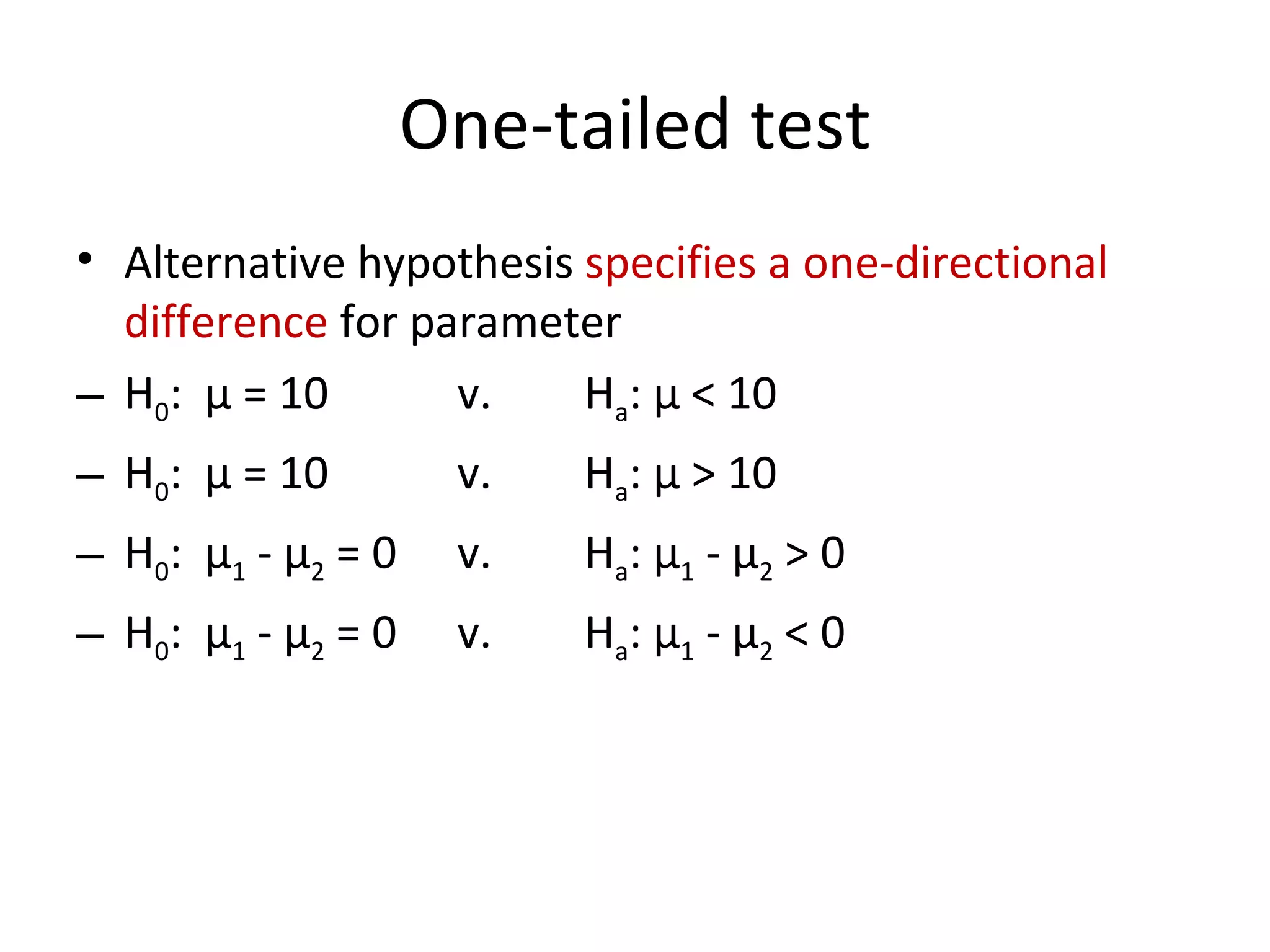
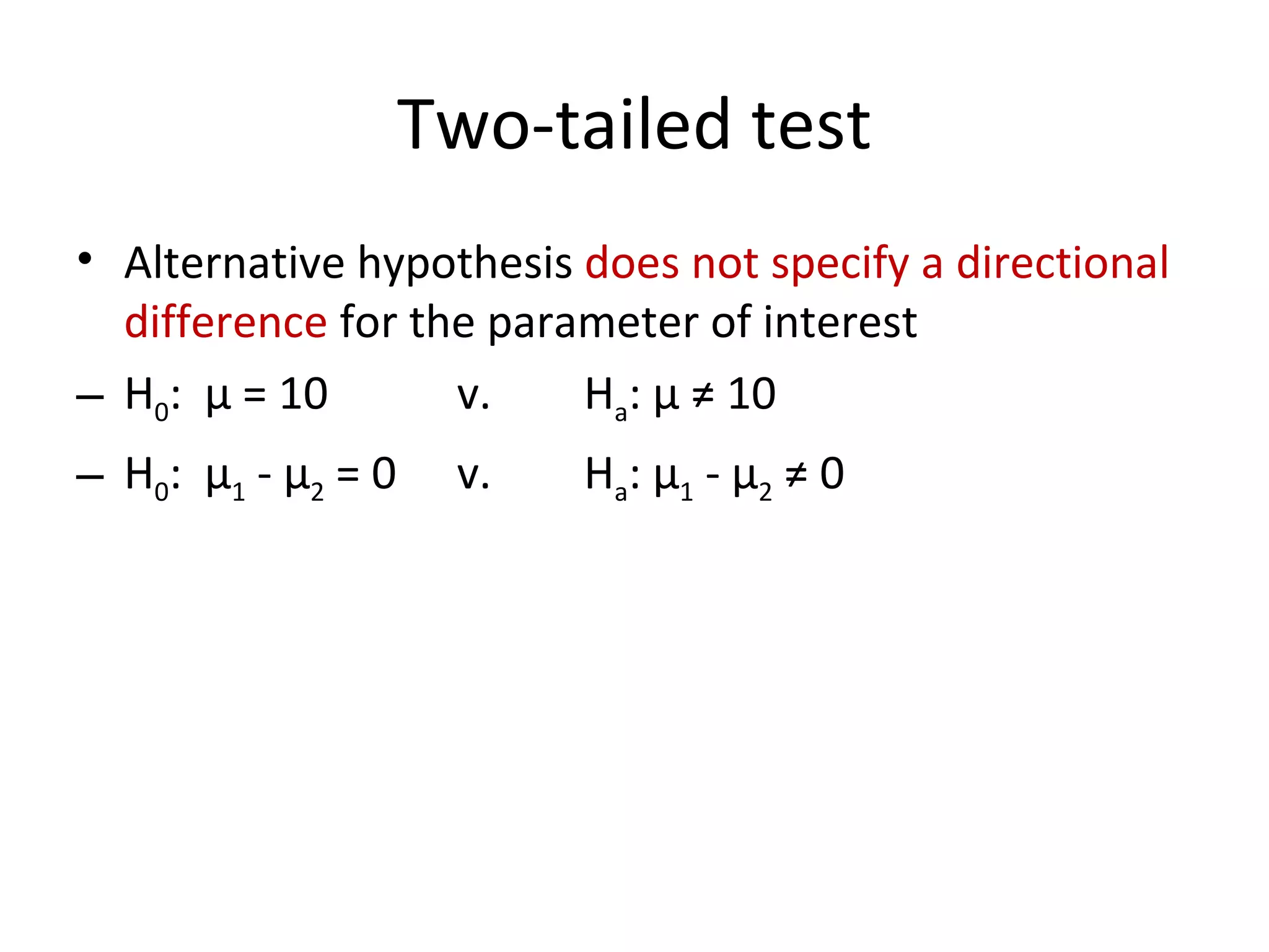
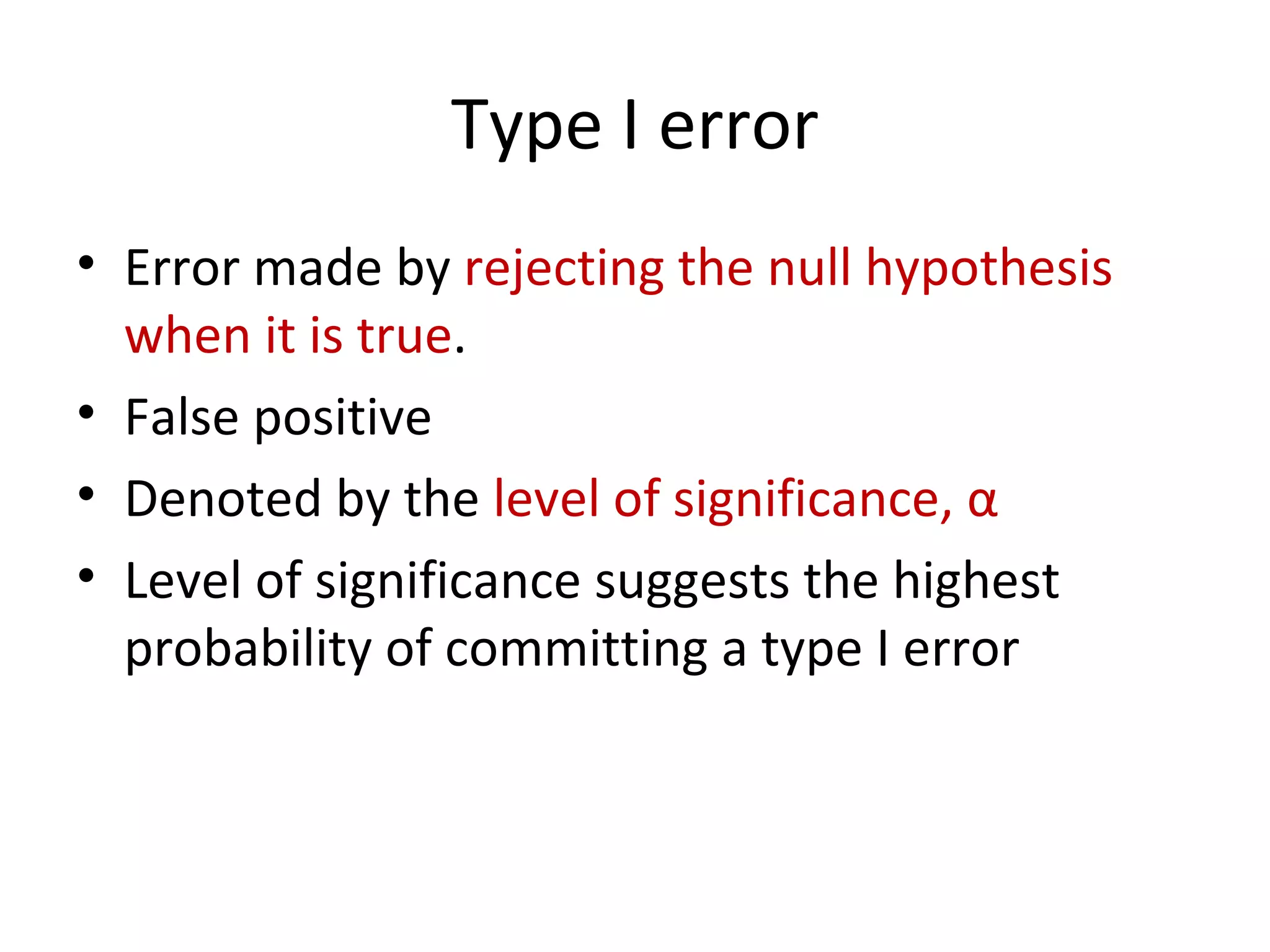
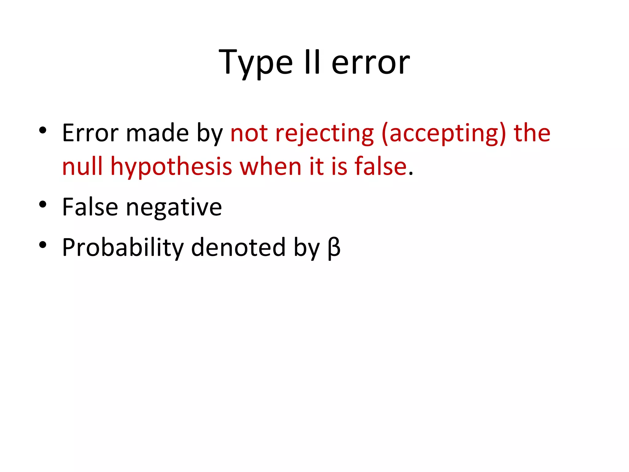
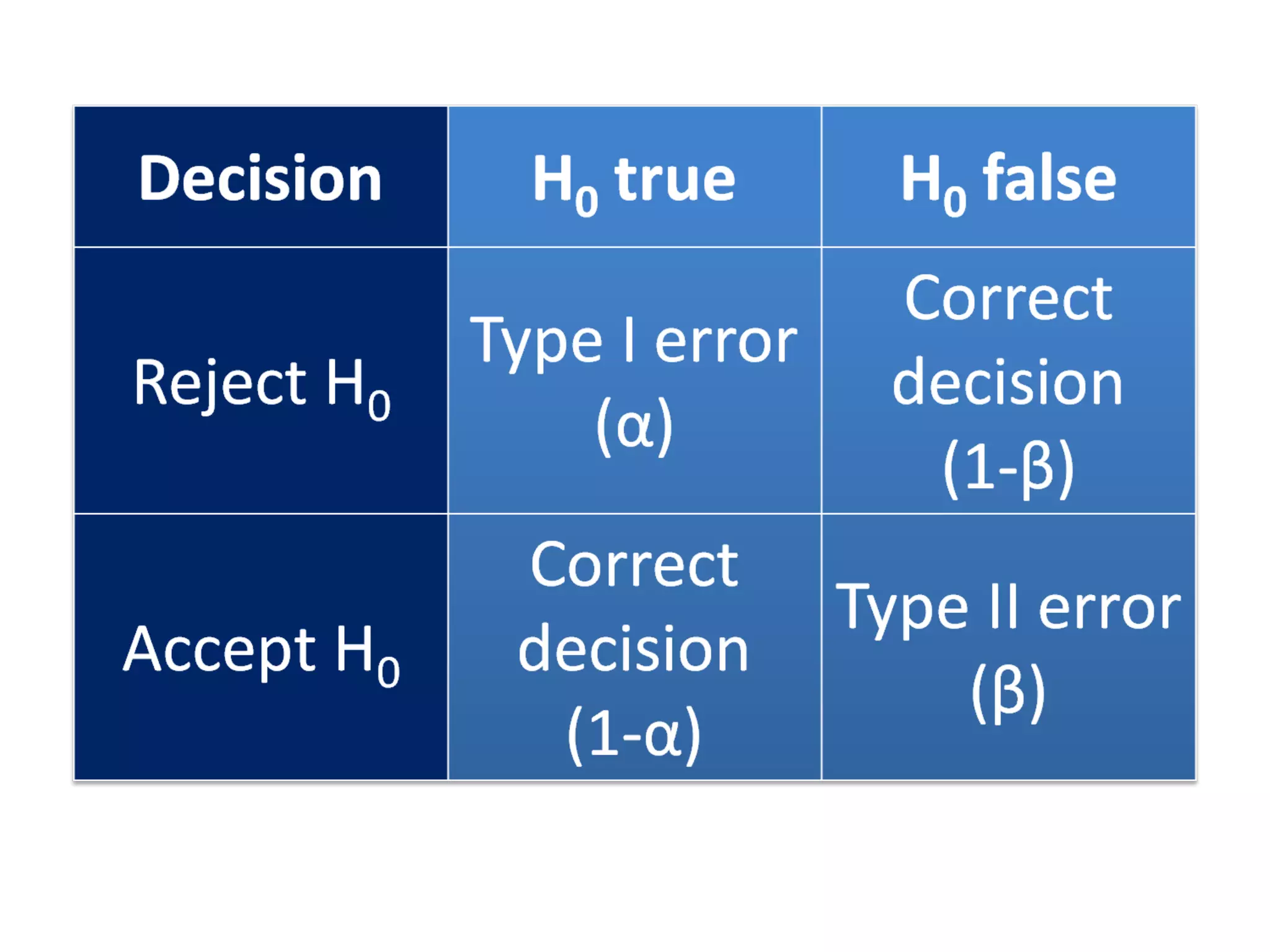
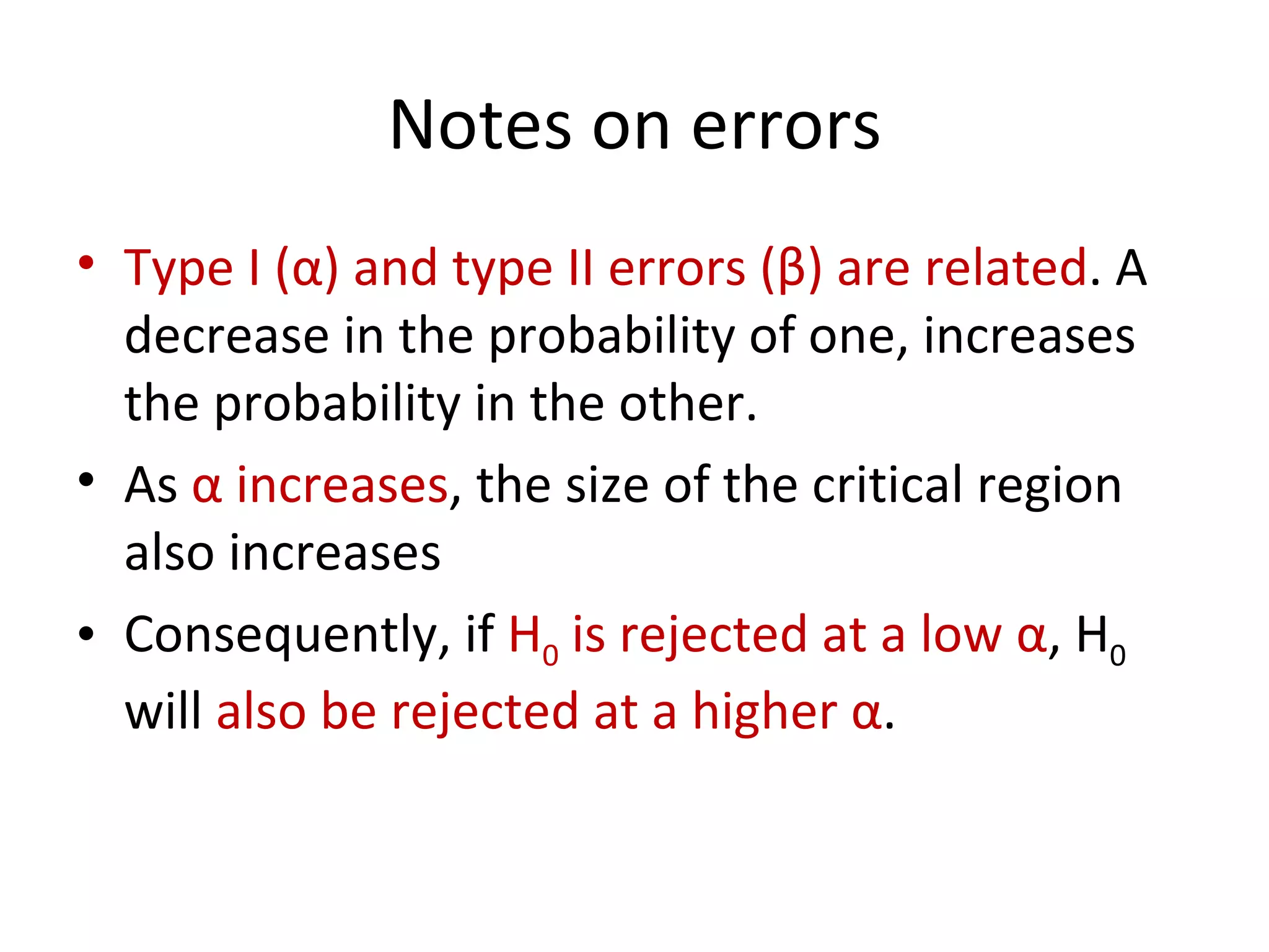
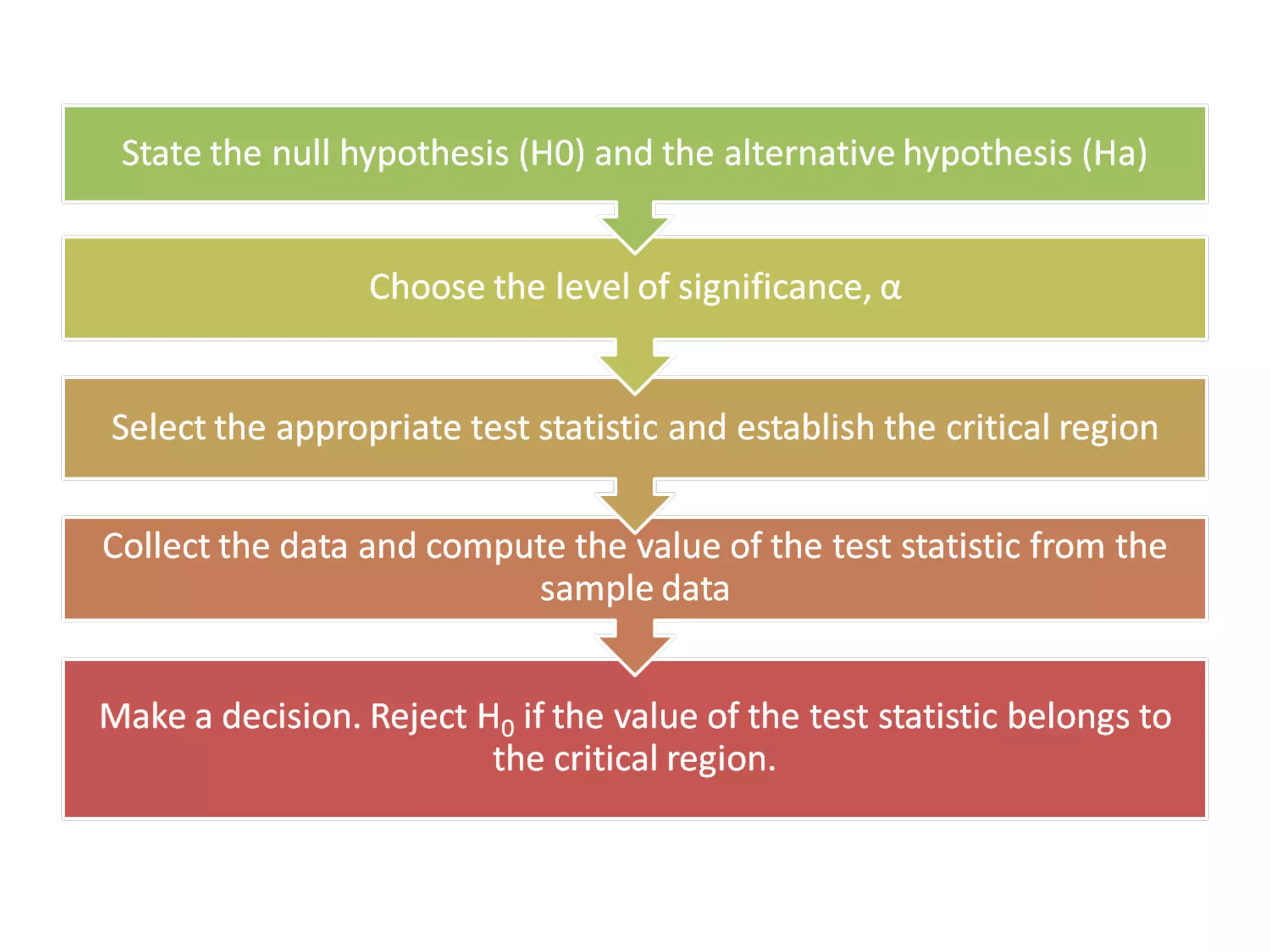
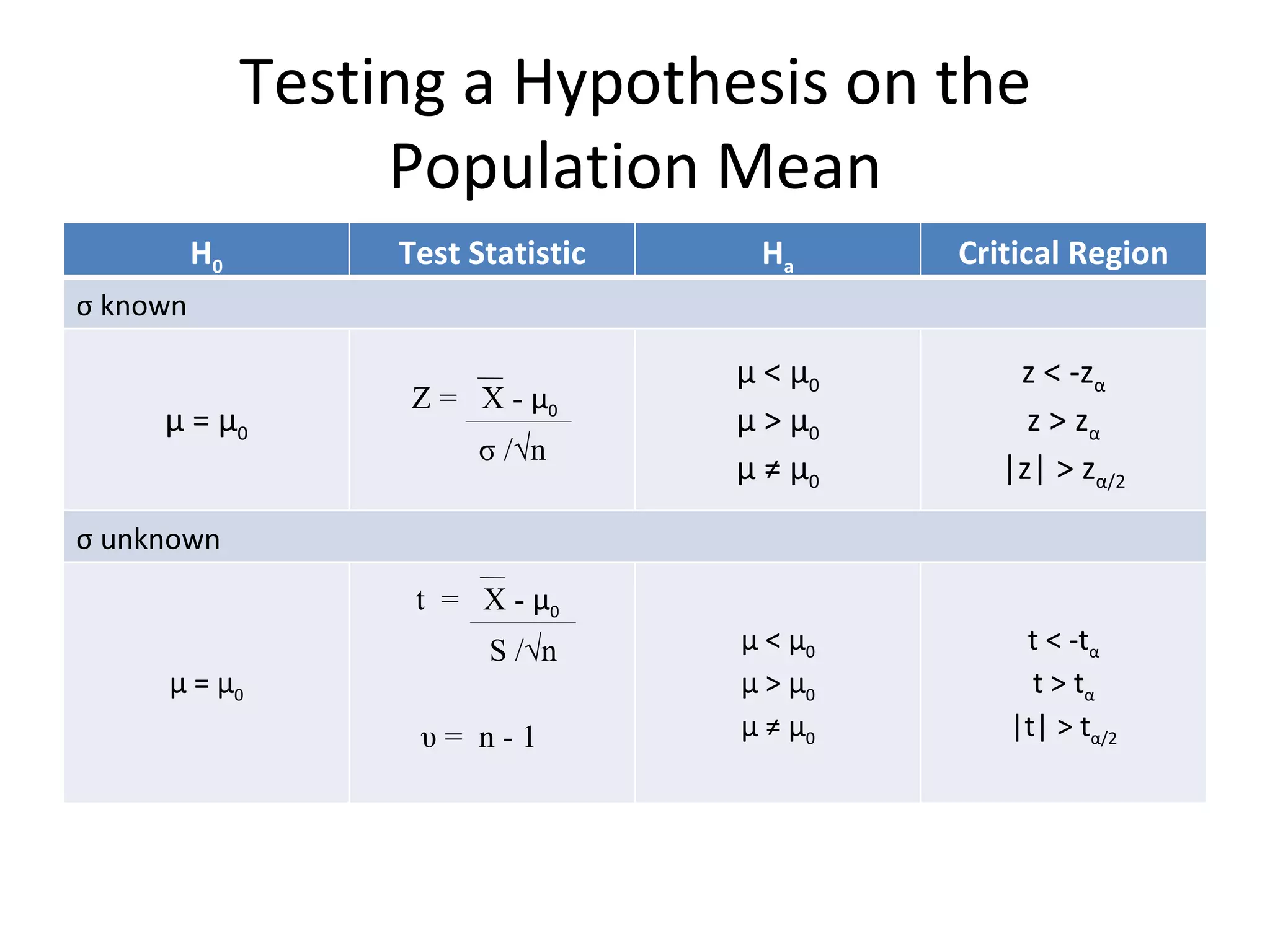
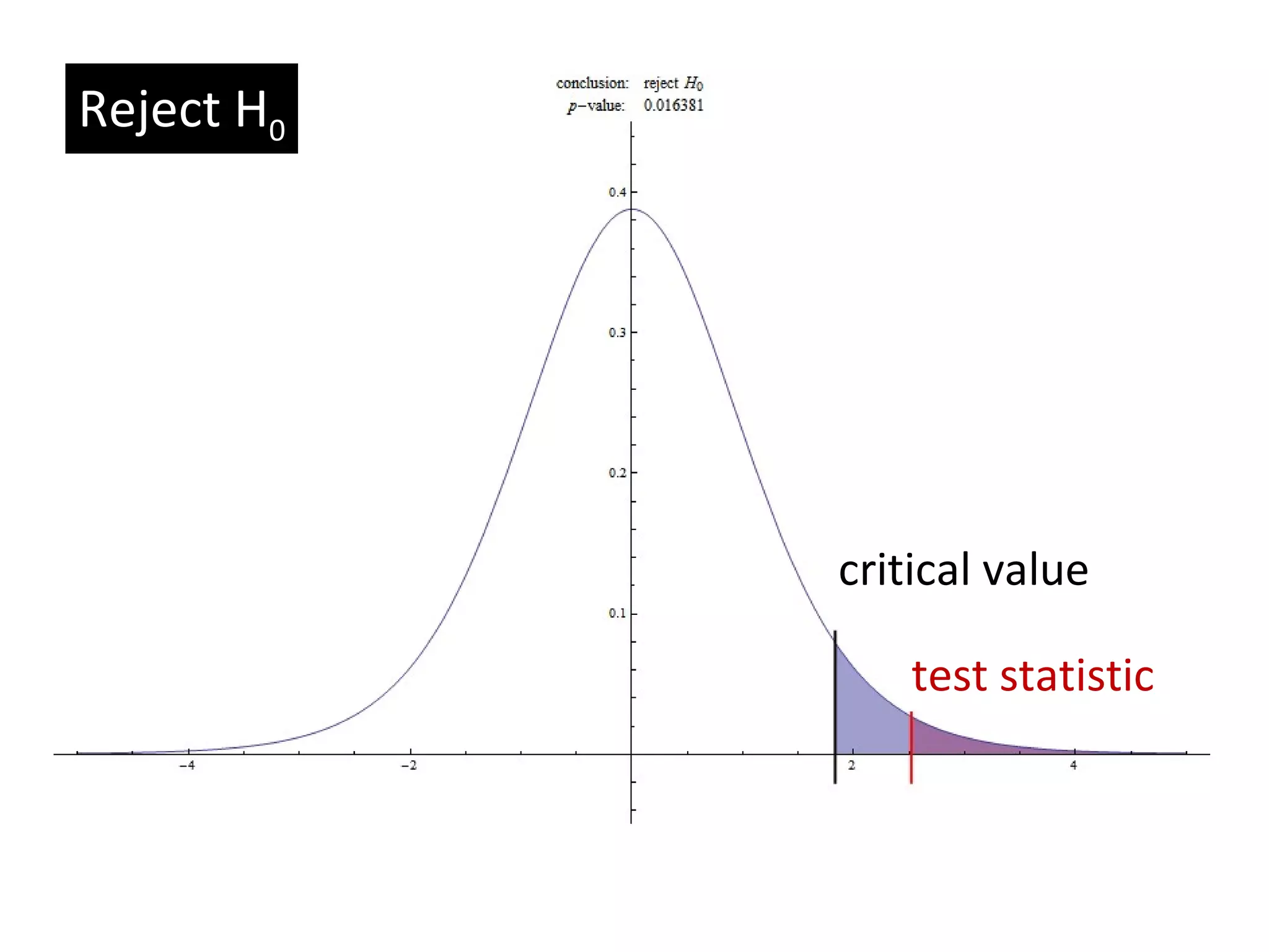
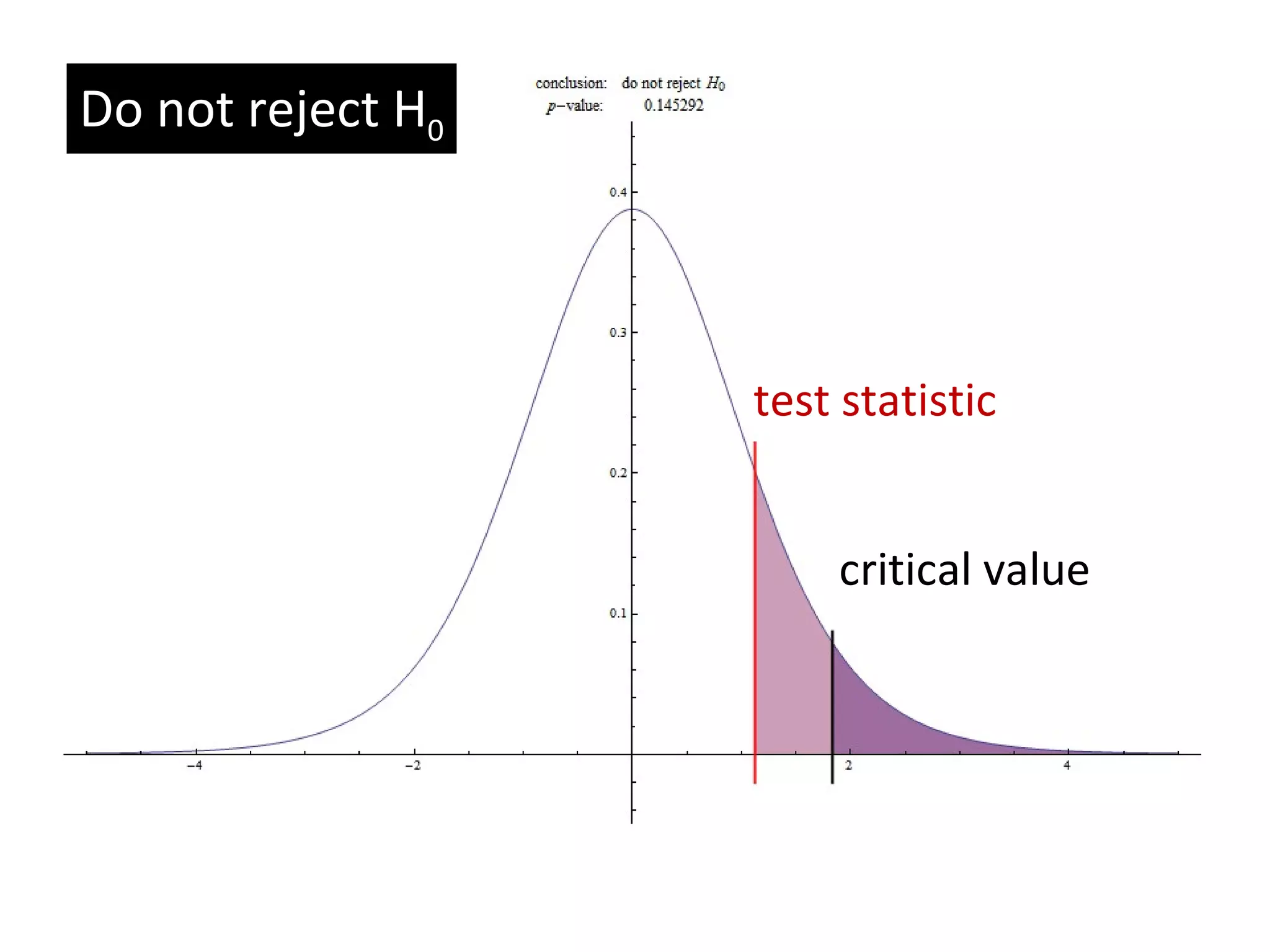
The document discusses the normal distribution and hypothesis testing. It provides characteristics of the normal distribution including its bell shape, mean, and percentages of observations within standard deviations of the mean. It also describes sampling distributions, the central limit theorem, and how the distribution of sample means approaches normality as sample size increases. Finally, it discusses hypothesis testing, including null and alternative hypotheses, types of tests, critical regions, types of errors, and how to test hypotheses about population means.

1. Normal Distribution and Hypothesis Testing STR1K

3. Characteristics Bell-shaped , depends on standard deviation Continuous distribution Unimodal Symmetric about the vertical axis through the mean μ Approaches the horizontal axis asymptotically Total area under the curve and above the horizontal is 1

4. Characteristics Approximately 68% of observations fall within 1 σ from the mean Approximately 95% of observations fall within 2 σ from the mean Approximately 99.7% of observations fall within 3 σ from the mean

5. 68.27% 95.45 % 99.73%

6. Standard Normal Distribution Special type of normal distribution where μ =0 Used to avoid integral calculus to find the area under the curve Standardizes raw data Dimensionless Z-score Z = X - μ 0 σ

7. Example 1 Given the normal distribution with μ = 49 and σ = 8, find the probability that X assumes a value: Less than 45 More than 50

8. Example 2 The achievement sores for a college entrance examination are normally distributed with the mean 75 and standard deviation equal to 10. What fraction of the scores would one expect to lie between 70 and 90.

9. Sampling Distribution Distribution of all possible sample statistics Population All Possible Samples Sample Means 1, 2, 3, 4 1, 2, 3 2.00 1, 2, 4 2.33 3, 4, 1 2.67 2, 3, 4 3.00 μ = 2.5; σ = 1.18 n = 3 μ xbar = 2.5

10. Central Limit Theorem Given a distribution with a mean μ and variance σ² , the sampling distribution of the mean approaches a normal distribution with a mean (μ) and a variance σ²/N as N, the sample size, increases.

11. Characteristics The mean of the population and the mean of the sampling distribution of means will always have the same value . The sampling distribution of the mean will be normal regardless of the shape of the population distribution.

12. N(70, 16)

13. N(70,1)

14. N(70,.25)

15. Characteristics As the sample size increases , the distribution of the sample average becomes less and less variable. Hence the sample average X bar approaches the value of the population mean μ .

16. Example 3 An electrical firm manufactures light bulbs that have a length of life normally distributed with mean and standard deviation equal to 500 and 50 hours respectively. Find the probability that a random sample of 15 bulbs will have an average life ofless than 475 hours.

17. HYPOTHESIS TESTING Normal Distribution and Hypothesis Testing

18. Hypothesis Testing A hypothesis is a conjecture or assertion about a parameter Null v. Alternative hypothesis Proof by contradiction Null hypothesis is the hypothesis being tested Alternative hypothesis is the operational statement of the experiment that is believed to be true

19. One-tailed test Alternative hypothesis specifies a one-directional difference for parameter H 0 : μ = 10 v. H a : μ < 10 H 0 : μ = 10 v. H a : μ > 10 H 0 : μ 1 - μ 2 = 0 v. H a : μ 1 - μ 2 > 0 H 0 : μ 1 - μ 2 = 0 v. H a : μ 1 - μ 2 < 0

20. Two-tailed test Alternative hypothesis does not specify a directional difference for the parameter of interest H 0 : μ = 10 v. H a : μ ≠ 10 H 0 : μ 1 - μ 2 = 0 v. H a : μ 1 - μ 2 ≠ 0

21. Critical Region Also known as the “rejection region” Critical region contains values of the test statistic for which the null hypothesis will be rejected Acceptance and rejection regions are separated by the critical value, Z .

22. Type I error Error made by rejecting the null hypothesis when it is true . False positive Denoted by the level of significance, α Level of significance suggests the highest probability of committing a type I error

23. Type II error Error made by not rejecting (accepting) the null hypothesis when it is false . False negative Probability denoted by β

25. Notes on errors Type I ( α ) and type II errors ( β ) are related . A decrease in the probability of one, increases the probability in the other. As α increases , the size of the critical region also increases Consequently, if H 0 is rejected at a low α , H 0 will also be rejected at a higher α .

27. Testing a Hypothesis on the Population Mean Z = X - μ 0 σ /√n t = X - μ 0 S /√n υ = n - 1 H 0 Test Statistic H a Critical Region σ known μ = μ 0 μ < μ 0 μ > μ 0 μ ≠ μ 0 z < -z α z > z α |z| > z α /2 σ unknown μ = μ 0 μ < μ 0 μ > μ 0 μ ≠ μ 0 t < -t α t > t α |t| > t α /2

28. critical value test statistic Reject H 0

29. critical value test statistic Do not reject H 0

30. Example 4 It is claimed that an automobile is driven on the average of less than 25,000 km per year. To test this claim, a random sample of 100 automobile owners are asked to keep a record of the kilometers they travel. Would you agree with this claim if the random sample showed an average of 23,500 km and a standard deviation of 3,900 km? Use 0.01 level of significance.