Downloaded 18 times
![Has a sample size below 30,
Has an unknown population standard deviation.
You must know the standard deviation of the population and your sample size
should be above 30 in order for you to be able to use the z-score. Otherwise, use the
t-score.
Z-score
Technically, z-scores are a conversion of individual scores into a standard form. The
conversion allows you to more easily compare different data. A z-score tells you how
many standard deviations from the mean your result is. You can use your knowledge
of normal distributions (like the 68 95 and 99.7 rule) or the z-table to determine
what percentage of the population will fall below or above your result.
The z-score is calculated using the formula:
● z = (X-μ)/σ
Where:
● σ is the population standard deviation and
● μ is the population mean.
● The z-score formula doesn’t say anything about sample size; The rule of thumb
applies that your sample size should be above 30 to use it.
T-score
Like z-scores, t-scores are also a conversion of individual scores into a standard form.
However, t-scores are used when you don’t know the population standard deviation;
You make an estimate by using your sample.
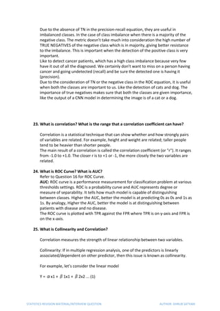
● T = (X – μ) / [ s/√(n) ]
Where:
● s is the standard deviation of the sample.
If you have a larger sample (over 30), the t-distribution and z-distribution look pretty
much the same.
To know more about Data Science, Artificial Intelligence, Machine Learning and
Deep Learning programs visit our website www.learnbay.co
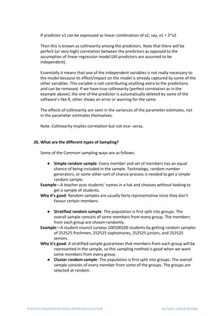
Follow us on:
LinkedIn
Facebook
Twitter
Watch our Live Session Recordings to precisely understand statistics, probability,
calculus, linear algebra and other math concepts used in data science.
Youtube
To get updates on Data Science and AI Seminars/Webinars - Follow our Meetup
group.
STATISTICS REVISION MATERIAL/INTERVIEW QUESTION AUTHOR: DHRUB SATYAM](https://image.slidesharecdn.com/interviewquestions-statistics-200528180758/85/Data-Science-interview-questions-of-Statistics-26-320.jpg)

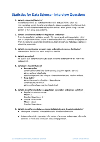
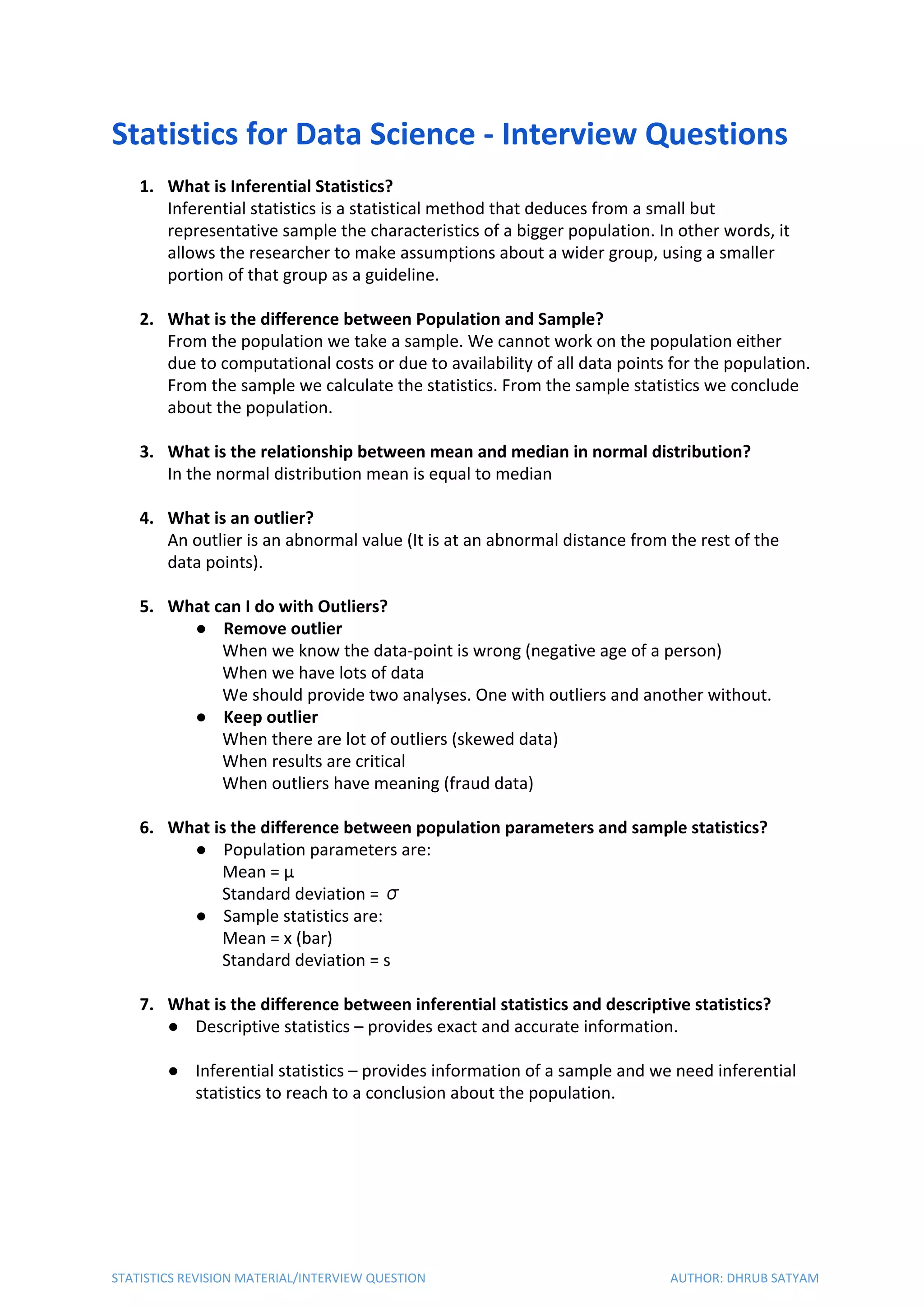
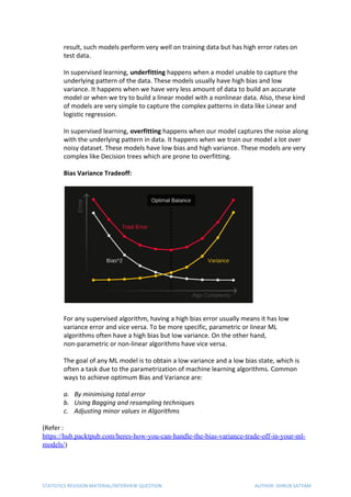
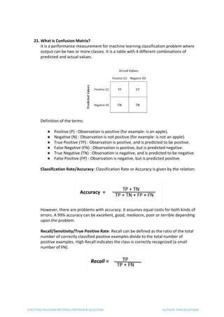
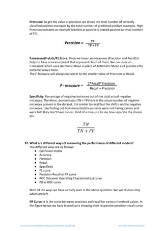
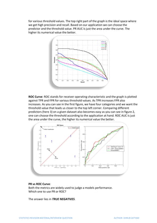
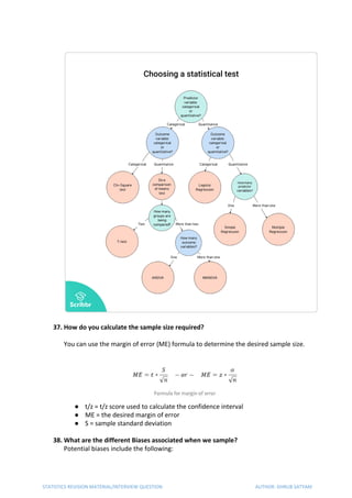
The document discusses key concepts in statistics relevant for data science, including definitions of inferential statistics, the relationship between population and samples, and the significance of mean, median, and outliers. It covers hypothesis testing, type I and type II errors, and methods to identify outliers using techniques such as z-scores and the interquartile range. The document serves as a revision guide for common statistics interview questions authored by Dhrub Satyam.