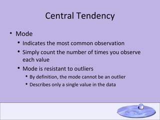
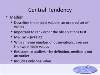
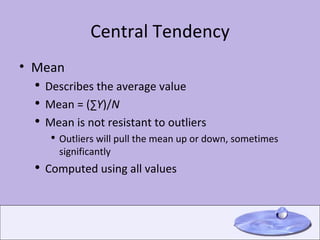
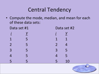
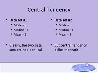
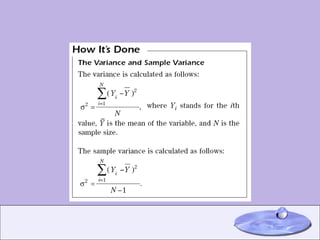
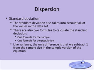
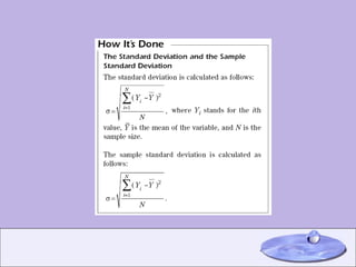
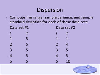
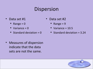
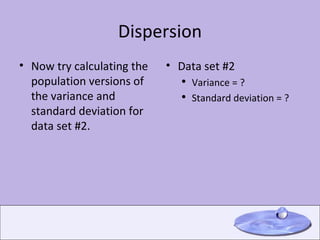
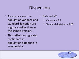
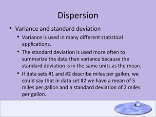
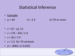
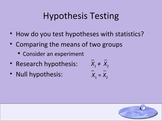
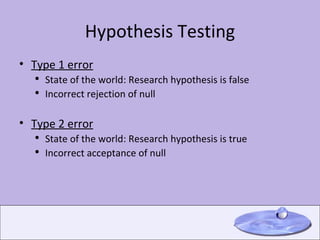
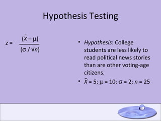
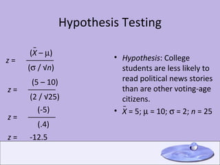
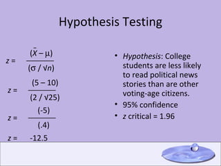
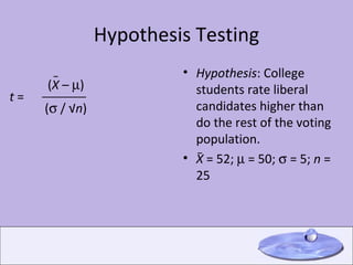
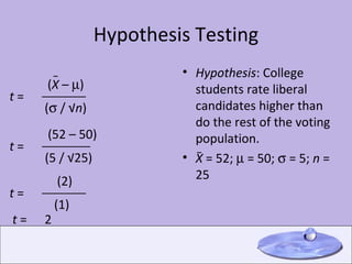
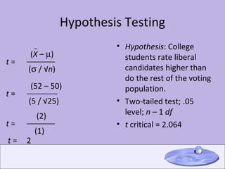
Chapter 11 Central Tendency Dispersion Statistical Inference Hypothesis Testing
Description We can describe data in a number of ways: We could describe every observation, or every value in a data set  (but this would be overwhelming and mostly unhelpful) Alternatively, we could summarize the data: Graphical summaries Bar graphs, pie graphs, dot plots, etc. Statistical summaries Frequency distributions Descriptive statistics
Description Frequency distributions A table that shows the number of observations having each value of a variable May include other statistics like the relative frequency proportion, percentage, missing values, or odds ratios Descriptive statistics Describing a large amount of data with just one number
Description Two classes of descriptive statistics Central tendency Dispersion
Central Tendency Measures of central tendency Describe the typical case in a data set or distribution Three statistics Mode Median Mean
Central Tendency Mode Indicates the most common observation Simply count the number of times you observe each value Mode is resistant to outliers By definition, the mode cannot be an outlier Describes only a single value in the data
Central Tendency Median Describes the middle value in an ordered set of values Important to rank order the observations first Median = ( N +1)/2  With an even number of observations, average the two middle values Resistant to outliers—by definition, median is not an outlier Includes only one value
Central Tendency Mean Describes the average value Mean = (∑ Y )/ N Mean is not resistant to outliers Outliers will pull the mean up or down, sometimes significantly Computed using all values
Central Tendency Compute the mode, median, and mean for each of these data sets: Data set #1 Data set #2 i Y i Y 1 5 1 1 2 5 2 4 3 5 3 5 4 5 4 5 5 5 5 10
Central Tendency Data set #1 Mode = 5 Median = 5 Mean = 5 Clearly, the two data sets are not identical Data set #2 Mode = 5 Median = 5 Mean = 5 But central tendency belies the truth
Dispersion What we need is some way to differentiate between data set #1 and data set #2. The typical values in each data set were the same. We need a measure that describes the other values in the data sets. Measures of dispersion indicate how the other values vary around the typical value.
Dispersion Measures of dispersion Range Variance Standard deviation
Dispersion Range One of the simplest measures of dispersion is the range. Range =  Y  maximum –  Y  minimum  Describes the extremes of the data around the typical case.
Dispersion Variance The variance takes into account all of the values in the data set. There are two formulas to calculate the variance: One formula for the sample One formula for the population The only difference is that we subtract 1 from the sample size in the sample version of the equation.
 
Dispersion Standard deviation The standard deviation also takes into account all of the values in the data set. There are also two formulas to calculate the standard deviation: One formula for the sample One formula for the population Like variance, the only difference is that we subtract 1 from the sample size in the sample version of the equation.
 
Dispersion Compute the range, sample variance, and sample standard deviation for each of these data sets: Data set #1 Data set #2 i Y i Y 1 5 1 1 2 5 2 4 3 5 3 5 4 5 4 5 5 5 5 10
Dispersion Data set #1 Range = 0 Variance = 0 Standard deviation = 0 Measures of dispersion indicate that the data sets are not the same. Data set #2 Range = 9 Variance = 10.5 Standard deviation = 3.24
Dispersion Now try calculating the population versions of the variance and standard deviation for data set #2. Data set #2 Variance = ? Standard deviation = ?
Dispersion As you can see, the population variance and standard deviation are slightly smaller than in the sample version. This reflects our greater confidence in population data than in sample data. Data set #2 Variance = 8.4 Standard deviation = 2.89
Dispersion Variance and standard deviation Variance is used in many different statistical applications. The standard deviation is used more often to summarize the data than variance because the standard deviation is in the same units as the mean. If data sets #1 and #2 describe miles per gallon, we could say that in data set #2 we have a mean of 5 miles per gallon and a standard deviation of 2 miles per gallon.
Statistical Inference The normal distribution is our first choice in most cases because it has such wonderful properties: Distribution is symmetrical around the mean Percentage of cases associated with standard deviations Can identify probability of values under the curve A linear combination of normally distributed variables is itself distributed normally Central limit theorem  Normal distribution is symmetric and mesokurtic   Great flexibility in using the normal distribution
Statistical Inference
Statistical Inference We can calculate a  z  score for every observation in the data set. The  z  score allows us to compare each observation to the rest of the data set, relative to the mean. z  score, or  z  of  X  =  ( X  –   )       
Statistical Inference Example :    = 64   = 2.4 X i =70 or more z  = ( X  –   ) /  
Statistical Inference Example :    = 64   = 2.4 X i =70 or more z  = ( X  –   ) /   z  = (70 – 64) / 2.4 z  = (6) / 2.4 z  = 2.5  for 70 contacts p = .0062; or 0.62%
Hypothesis Testing How do you test hypotheses with statistics? Comparing the means of two groups Consider an experiment Research hypothesis:  Null hypothesis: X 1  ≠  X 2   ─ ─ X 1  =  X 2 ─ ─
Hypothesis Testing Type 1 error State of the world: Research hypothesis is false Incorrect rejection of null Type 2 error State of the world: Research hypothesis is true Incorrect acceptance of null
Hypothesis Testing Hypothesis : College students are less likely to read political news stories than are other voting-age citizens.  X  = 5;    = 10;    = 2;  n  = 25  ( X  –   ) (   / √ n ) __________ z  =  _ _
Hypothesis Testing Hypothesis : College students are less likely to read political news stories than are other voting-age citizens.  X  = 5;    = 10;    = 2;  n  = 25  _ -12.5  z  =  ( X  –   ) (   / √ n ) __________ z  =  _ (5 – 10) (2 / √25) __________ z  =  (-5) (.4) __________ z  =
Hypothesis Testing Hypothesis : College students are less likely to read political news stories than are other voting-age citizens.  95% confidence z  critical = 1.96 -12.5  z  =  ( X  –   ) (   / √ n ) __________ z  =  _ (5 – 10) (2 / √25) __________ z  =  (-5) (.4) __________ z  =
Hypothesis Testing Hypothesis : College students rate liberal candidates higher than do the rest of the voting population.  X  = 52;    = 50;    = 5;  n  = 25 _ ( X  –   ) (   / √ n ) __________ t  =  _
Hypothesis Testing Hypothesis : College students rate liberal candidates higher than do the rest of the voting population.  X  = 52;    = 50;    = 5;  n  = 25 2  t  =  _ ( X  –   ) (   / √ n ) __________ t  =  _ (52 – 50) (5 / √25) ___________ t  =  (2) (1) __________ t  =
Hypothesis Testing Hypothesis : College students rate liberal candidates higher than do the rest of the voting population.  Two-tailed test; .05 level;  n  – 1  df t  critical = 2.064 2  t  =  ( X  –   ) (   / √ n ) __________ t  =  _ (52 – 50) (5 / √25) ___________ t  =  (2) (1) __________ t  =

Chapter 11 Psrm

  • 1.
    Chapter 11 CentralTendency Dispersion Statistical Inference Hypothesis Testing
  • 2.
    Description We candescribe data in a number of ways: We could describe every observation, or every value in a data set (but this would be overwhelming and mostly unhelpful) Alternatively, we could summarize the data: Graphical summaries Bar graphs, pie graphs, dot plots, etc. Statistical summaries Frequency distributions Descriptive statistics
  • 3.
    Description Frequency distributionsA table that shows the number of observations having each value of a variable May include other statistics like the relative frequency proportion, percentage, missing values, or odds ratios Descriptive statistics Describing a large amount of data with just one number
  • 4.
    Description Two classesof descriptive statistics Central tendency Dispersion
  • 5.
    Central Tendency Measuresof central tendency Describe the typical case in a data set or distribution Three statistics Mode Median Mean
  • 6.
    Central Tendency ModeIndicates the most common observation Simply count the number of times you observe each value Mode is resistant to outliers By definition, the mode cannot be an outlier Describes only a single value in the data
  • 7.
    Central Tendency MedianDescribes the middle value in an ordered set of values Important to rank order the observations first Median = ( N +1)/2 With an even number of observations, average the two middle values Resistant to outliers—by definition, median is not an outlier Includes only one value
  • 8.
    Central Tendency MeanDescribes the average value Mean = (∑ Y )/ N Mean is not resistant to outliers Outliers will pull the mean up or down, sometimes significantly Computed using all values
  • 9.
    Central Tendency Computethe mode, median, and mean for each of these data sets: Data set #1 Data set #2 i Y i Y 1 5 1 1 2 5 2 4 3 5 3 5 4 5 4 5 5 5 5 10
  • 10.
    Central Tendency Dataset #1 Mode = 5 Median = 5 Mean = 5 Clearly, the two data sets are not identical Data set #2 Mode = 5 Median = 5 Mean = 5 But central tendency belies the truth
  • 11.
    Dispersion What weneed is some way to differentiate between data set #1 and data set #2. The typical values in each data set were the same. We need a measure that describes the other values in the data sets. Measures of dispersion indicate how the other values vary around the typical value.
  • 12.
    Dispersion Measures ofdispersion Range Variance Standard deviation
  • 13.
    Dispersion Range Oneof the simplest measures of dispersion is the range. Range = Y maximum – Y minimum Describes the extremes of the data around the typical case.
  • 14.
    Dispersion Variance Thevariance takes into account all of the values in the data set. There are two formulas to calculate the variance: One formula for the sample One formula for the population The only difference is that we subtract 1 from the sample size in the sample version of the equation.
  • 15.
  • 16.
    Dispersion Standard deviationThe standard deviation also takes into account all of the values in the data set. There are also two formulas to calculate the standard deviation: One formula for the sample One formula for the population Like variance, the only difference is that we subtract 1 from the sample size in the sample version of the equation.
  • 17.
  • 18.
    Dispersion Compute therange, sample variance, and sample standard deviation for each of these data sets: Data set #1 Data set #2 i Y i Y 1 5 1 1 2 5 2 4 3 5 3 5 4 5 4 5 5 5 5 10
  • 19.
    Dispersion Data set#1 Range = 0 Variance = 0 Standard deviation = 0 Measures of dispersion indicate that the data sets are not the same. Data set #2 Range = 9 Variance = 10.5 Standard deviation = 3.24
  • 20.
    Dispersion Now trycalculating the population versions of the variance and standard deviation for data set #2. Data set #2 Variance = ? Standard deviation = ?
  • 21.
    Dispersion As youcan see, the population variance and standard deviation are slightly smaller than in the sample version. This reflects our greater confidence in population data than in sample data. Data set #2 Variance = 8.4 Standard deviation = 2.89
  • 22.
    Dispersion Variance andstandard deviation Variance is used in many different statistical applications. The standard deviation is used more often to summarize the data than variance because the standard deviation is in the same units as the mean. If data sets #1 and #2 describe miles per gallon, we could say that in data set #2 we have a mean of 5 miles per gallon and a standard deviation of 2 miles per gallon.
  • 23.
    Statistical Inference Thenormal distribution is our first choice in most cases because it has such wonderful properties: Distribution is symmetrical around the mean Percentage of cases associated with standard deviations Can identify probability of values under the curve A linear combination of normally distributed variables is itself distributed normally Central limit theorem Normal distribution is symmetric and mesokurtic Great flexibility in using the normal distribution
  • 24.
  • 25.
    Statistical Inference Wecan calculate a z score for every observation in the data set. The z score allows us to compare each observation to the rest of the data set, relative to the mean. z score, or z of X = ( X –  ) 
  • 26.
    Statistical Inference Example:  = 64  = 2.4 X i =70 or more z = ( X –  ) / 
  • 27.
    Statistical Inference Example:  = 64  = 2.4 X i =70 or more z = ( X –  ) /  z = (70 – 64) / 2.4 z = (6) / 2.4 z = 2.5 for 70 contacts p = .0062; or 0.62%
  • 28.
    Hypothesis Testing Howdo you test hypotheses with statistics? Comparing the means of two groups Consider an experiment Research hypothesis: Null hypothesis: X 1 ≠ X 2 ─ ─ X 1 = X 2 ─ ─
  • 29.
    Hypothesis Testing Type1 error State of the world: Research hypothesis is false Incorrect rejection of null Type 2 error State of the world: Research hypothesis is true Incorrect acceptance of null
  • 30.
    Hypothesis Testing Hypothesis: College students are less likely to read political news stories than are other voting-age citizens. X = 5;  = 10;  = 2; n = 25 ( X –  ) (  / √ n ) __________ z = _ _
  • 31.
    Hypothesis Testing Hypothesis: College students are less likely to read political news stories than are other voting-age citizens. X = 5;  = 10;  = 2; n = 25 _ -12.5 z = ( X –  ) (  / √ n ) __________ z = _ (5 – 10) (2 / √25) __________ z = (-5) (.4) __________ z =
  • 32.
    Hypothesis Testing Hypothesis: College students are less likely to read political news stories than are other voting-age citizens. 95% confidence z critical = 1.96 -12.5 z = ( X –  ) (  / √ n ) __________ z = _ (5 – 10) (2 / √25) __________ z = (-5) (.4) __________ z =
  • 33.
    Hypothesis Testing Hypothesis: College students rate liberal candidates higher than do the rest of the voting population. X = 52;  = 50;  = 5; n = 25 _ ( X –  ) (  / √ n ) __________ t = _
  • 34.
    Hypothesis Testing Hypothesis: College students rate liberal candidates higher than do the rest of the voting population. X = 52;  = 50;  = 5; n = 25 2 t = _ ( X –  ) (  / √ n ) __________ t = _ (52 – 50) (5 / √25) ___________ t = (2) (1) __________ t =
  • 35.
    Hypothesis Testing Hypothesis: College students rate liberal candidates higher than do the rest of the voting population. Two-tailed test; .05 level; n – 1 df t critical = 2.064 2 t = ( X –  ) (  / √ n ) __________ t = _ (52 – 50) (5 / √25) ___________ t = (2) (1) __________ t =