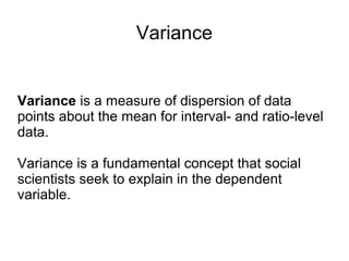
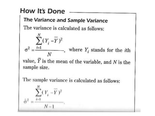
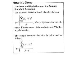
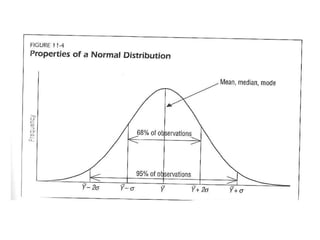
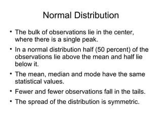
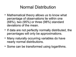
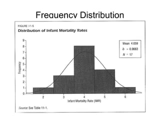
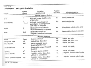
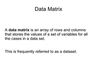
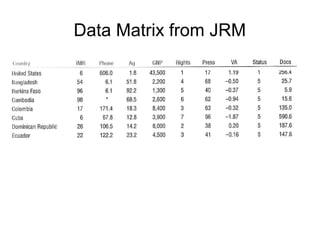
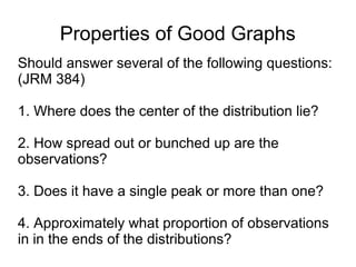
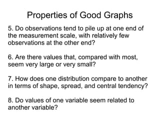
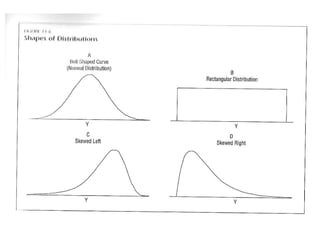
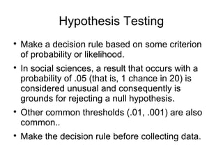
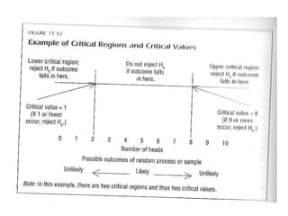
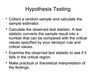
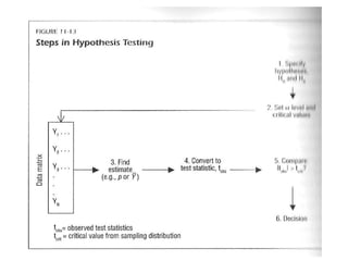
Statistics: First Steps
Andrew Martin
PS 372
University of Kentucky
Variance
Variance is a measure of dispersion of data
points about the mean for interval- and ratio-level
data.
Variance is a fundamental concept that social
scientists seek to explain in the dependent
variable.
Standard Deviation
Standard deviation is a measure of dispersion of
data points about the mean for interval- and ratio-
level data.
Like the mean, standard deviation is sensitive to
extreme values.
Standard deviation is calculated as the square
root of the variance.
Normal Distribution

The bulk of observations lie in the center,
where there is a single peak.

In a normal distribution half (50 percent) of the
observations lie above the mean and half lie
below it.

The mean, median and mode have the same
statistical values.

Fewer and fewer observations fall in the tails.

The spread of the distribution is symmetric.
Normal Distribution

Mathematical theory allows us to know what
percentage of observations lie within one
(68%), two (95%) or three (98%) standard
deviations of the mean.

If data are not perfectly normally distributed, the
percentages will only be approximations.

Many naturally occurring variables do have
nearly normal distributions.

Some can be transformed using logarithms.
Frequency Distribution
What about categorical variables?
Example
Calculate the ID and IQV for a former PS 372
class grades using the following frequencies or
proportions:
Grade Freq. Prop.
A 4 (.12)
B 7 (.21)
C 4 (.12)
D 7 (.21)
E 12 (.34)
Index of Diversity
ID = 1 – (p2
a
+ p2
b
+ p2
c
+p2
d
+p2
e
)
ID = 1 - (.122
+ .212
+ .122
+ .212
+ .342
)
ID = 1 - (.0144 + .0441 + .0144 + .0441 + .1156)
ID = 1 - (.2326)
ID = .7674
Index of Qualitative Variation
1 – (p2
a
+ p2
b
+ p2
c
+p2
d
+p2
e
)
1 - (1/K)
Index of Qualitative Variation
.7674
(1 – 1/5)
.9592
Data Matrix
A data matrix is an array of rows and columns
that stores the values of a set of variables for all
the cases in a data set.
This is frequently referred to as a dataset.
Data Matrix from JRM
Properties of Good Graphs
Should answer several of the following questions:
(JRM 384)
1. Where does the center of the distribution lie?
2. How spread out or bunched up are the
observations?
3. Does it have a single peak or more than one?
4. Approximately what proportion of observations
in in the ends of the distributions?
Properties of Good Graphs
5. Do observations tend to pile up at one end of
the measurement scale, with relatively few
observations at the other end?
6. Are there values that, compared with most,
seem very large or very small?
7. How does one distribution compare to another
in terms of shape, spread, and central tendency?
8. Do values of one variable seem related to
another variable?
Statistical Concepts
Let's quickly review some concepts.
Population
A population refers to any well-defined set of
objects such as people, countries, states,
organizations, and so on. The term doesn't simply
mean the population of the United States or some
other geographical area.
Population

A sample is a subset of the population.

Samples are drawn in some known manner and
each case is chosen independently of the other.

From here on out, when the book uses the term
sample, random sample or simple random
sample, it's making reference to the same
concept, which is a sample chosen at random.
Populations

Parameters are numerical features of a
population.

A sample statistic is an estimator that
corresponds to a population parameter of
interest and is used to estimate the population
value.

Y is the sample mean, (μ) is the population
mean.

^ is a “hat”, caret or circumflex
Two Kinds of Inference
Hypothesis Testing
Point and interval estimation
Hypothesis Testing
Many claims can be translated into specific
statements about a population that can be
confirmed or disconfirmed with the aid of
probability theory.
Ex: There is no ideological difference between the
voting patterns between the voting patterns of
Republican and Democrat justices on the U.S.
Supreme Court.
Point and Interval Estimation
The goal here is to estimate unknown population
parameters from samples and to surround those
estimates with confidence intervals. Confidence
intervals suggest the estimates reliability or
precision.
Hypothesis Testing
Start with a specific verbal claim or proposition.
Ex: The chances of getting heads or tails when
flipping the coin is are roughly the same.
Ex: The chances of the United States electing a
Republican or Democrat president are roughly the
same.
Hypothesis Testing
Hypothesis Testing
Next, the researcher constructs a null hypothesis.
A null hypothesis is a statement that a
population parameter equals a specific value.
Hypothesis Testing
Following up on the coin example, the null
hypothesis would equal .5.
Stated more formally: H0
: P = .5
Where P stands for the probability that the coin
will be heads when tossed.
H0
is typically used to denote a null hypothesis.
Hypothesis Testing

Next, specify an alternative hypothesis.

An alternative hypothesis is a statement
about the value or values of a population
parameter. It is proposed as an alternative to
the null hypothesis.

An alternative hypothesis can merely state that
the population does not equal the null
hypothesis, or is greater than or less than the
null hypothesis.
Hypothesis Testing
Suppose you believe the coin is unfair, but have
no intuition about whether it is too prone to come
up heads or tails.
Stated formally, the alternative hypothesis is:
HA
: P ≠ .5
Hypothesis Testing
Perhaps you believe the coin is more likely to
come up heads than tails. You would formulate
the following alternative hypothesis:
HA
: P > .5
Conversely, if you believe the coin is less likely to
come up heads than tails, you would formulate
the alternative hypothesis in the opposite
direction:
HA
: P < .5
Hypothesis Testing

After specifying the null and alternative
hypothesis, identify the sample estimator that
corresponds to the parameter in question.

The sample must come from the data, which in
this case is generated by flipping a coin.
Hypothesis Testing

Next, determine how the sample statistic is
distributed in repeated random samples. That
is, specify the sampling distribution of the
estimator.

For example, what are the chances of getting
10 heads in 10 flips (p = 1.)? What about 9
heads in 10 flips (p = .9)? 8 flips (p = .8)?
Hypothesis Testing

Make a decision rule based on some criterion
of probability or likelihood.

In social sciences, a result that occurs with a
probability of .05 (that is, 1 chance in 20) is
considered unusual and consequently is
grounds for rejecting a null hypothesis.

Other common thresholds (.01, .001) are also
common..

Make the decision rule before collecting data.
Hypothesis Testing

In light of the decision rule, define a critical
region. The critical region consists of those
outcomes so unlikely to occur that one has
cause to reject the null hypothesis should they
occur.

So there are areas of “rejection” (critical areas)
and nonrejection.
Hypothesis Testing

Collect a random sample and calculate the
sample estimator.

Calculate the observed test statistic. A test
statistic converts the sample result into a
number that can be compared with the critical
values specified by your decision rule and
critical values.

Examine the observed test statistic to see if it
falls in the critical region.

Make practical or theoretical interpretation of
the findings.
Statistics 091208004734-phpapp01 (1)

Statistics 091208004734-phpapp01 (1)

  • 1.
    Statistics: First Steps AndrewMartin PS 372 University of Kentucky
  • 2.
    Variance Variance is ameasure of dispersion of data points about the mean for interval- and ratio-level data. Variance is a fundamental concept that social scientists seek to explain in the dependent variable.
  • 4.
    Standard Deviation Standard deviationis a measure of dispersion of data points about the mean for interval- and ratio- level data. Like the mean, standard deviation is sensitive to extreme values. Standard deviation is calculated as the square root of the variance.
  • 7.
    Normal Distribution  The bulkof observations lie in the center, where there is a single peak.  In a normal distribution half (50 percent) of the observations lie above the mean and half lie below it.  The mean, median and mode have the same statistical values.  Fewer and fewer observations fall in the tails.  The spread of the distribution is symmetric.
  • 8.
    Normal Distribution  Mathematical theoryallows us to know what percentage of observations lie within one (68%), two (95%) or three (98%) standard deviations of the mean.  If data are not perfectly normally distributed, the percentages will only be approximations.  Many naturally occurring variables do have nearly normal distributions.  Some can be transformed using logarithms.
  • 9.
  • 10.
  • 12.
    Example Calculate the IDand IQV for a former PS 372 class grades using the following frequencies or proportions: Grade Freq. Prop. A 4 (.12) B 7 (.21) C 4 (.12) D 7 (.21) E 12 (.34)
  • 13.
    Index of Diversity ID= 1 – (p2 a + p2 b + p2 c +p2 d +p2 e ) ID = 1 - (.122 + .212 + .122 + .212 + .342 ) ID = 1 - (.0144 + .0441 + .0144 + .0441 + .1156) ID = 1 - (.2326) ID = .7674
  • 14.
    Index of QualitativeVariation 1 – (p2 a + p2 b + p2 c +p2 d +p2 e ) 1 - (1/K)
  • 15.
    Index of QualitativeVariation .7674 (1 – 1/5) .9592
  • 17.
    Data Matrix A datamatrix is an array of rows and columns that stores the values of a set of variables for all the cases in a data set. This is frequently referred to as a dataset.
  • 20.
  • 21.
    Properties of GoodGraphs Should answer several of the following questions: (JRM 384) 1. Where does the center of the distribution lie? 2. How spread out or bunched up are the observations? 3. Does it have a single peak or more than one? 4. Approximately what proportion of observations in in the ends of the distributions?
  • 22.
    Properties of GoodGraphs 5. Do observations tend to pile up at one end of the measurement scale, with relatively few observations at the other end? 6. Are there values that, compared with most, seem very large or very small? 7. How does one distribution compare to another in terms of shape, spread, and central tendency? 8. Do values of one variable seem related to another variable?
  • 28.
  • 29.
    Population A population refersto any well-defined set of objects such as people, countries, states, organizations, and so on. The term doesn't simply mean the population of the United States or some other geographical area.
  • 30.
    Population  A sample isa subset of the population.  Samples are drawn in some known manner and each case is chosen independently of the other.  From here on out, when the book uses the term sample, random sample or simple random sample, it's making reference to the same concept, which is a sample chosen at random.
  • 31.
    Populations  Parameters are numericalfeatures of a population.  A sample statistic is an estimator that corresponds to a population parameter of interest and is used to estimate the population value.  Y is the sample mean, (μ) is the population mean.  ^ is a “hat”, caret or circumflex
  • 32.
    Two Kinds ofInference Hypothesis Testing Point and interval estimation
  • 33.
    Hypothesis Testing Many claimscan be translated into specific statements about a population that can be confirmed or disconfirmed with the aid of probability theory. Ex: There is no ideological difference between the voting patterns between the voting patterns of Republican and Democrat justices on the U.S. Supreme Court.
  • 34.
    Point and IntervalEstimation The goal here is to estimate unknown population parameters from samples and to surround those estimates with confidence intervals. Confidence intervals suggest the estimates reliability or precision.
  • 35.
    Hypothesis Testing Start witha specific verbal claim or proposition. Ex: The chances of getting heads or tails when flipping the coin is are roughly the same. Ex: The chances of the United States electing a Republican or Democrat president are roughly the same.
  • 36.
  • 37.
    Hypothesis Testing Next, theresearcher constructs a null hypothesis. A null hypothesis is a statement that a population parameter equals a specific value.
  • 38.
    Hypothesis Testing Following upon the coin example, the null hypothesis would equal .5. Stated more formally: H0 : P = .5 Where P stands for the probability that the coin will be heads when tossed. H0 is typically used to denote a null hypothesis.
  • 39.
    Hypothesis Testing  Next, specifyan alternative hypothesis.  An alternative hypothesis is a statement about the value or values of a population parameter. It is proposed as an alternative to the null hypothesis.  An alternative hypothesis can merely state that the population does not equal the null hypothesis, or is greater than or less than the null hypothesis.
  • 40.
    Hypothesis Testing Suppose youbelieve the coin is unfair, but have no intuition about whether it is too prone to come up heads or tails. Stated formally, the alternative hypothesis is: HA : P ≠ .5
  • 41.
    Hypothesis Testing Perhaps youbelieve the coin is more likely to come up heads than tails. You would formulate the following alternative hypothesis: HA : P > .5 Conversely, if you believe the coin is less likely to come up heads than tails, you would formulate the alternative hypothesis in the opposite direction: HA : P < .5
  • 42.
    Hypothesis Testing  After specifyingthe null and alternative hypothesis, identify the sample estimator that corresponds to the parameter in question.  The sample must come from the data, which in this case is generated by flipping a coin.
  • 43.
    Hypothesis Testing  Next, determinehow the sample statistic is distributed in repeated random samples. That is, specify the sampling distribution of the estimator.  For example, what are the chances of getting 10 heads in 10 flips (p = 1.)? What about 9 heads in 10 flips (p = .9)? 8 flips (p = .8)?
  • 45.
    Hypothesis Testing  Make adecision rule based on some criterion of probability or likelihood.  In social sciences, a result that occurs with a probability of .05 (that is, 1 chance in 20) is considered unusual and consequently is grounds for rejecting a null hypothesis.  Other common thresholds (.01, .001) are also common..  Make the decision rule before collecting data.
  • 46.
    Hypothesis Testing  In lightof the decision rule, define a critical region. The critical region consists of those outcomes so unlikely to occur that one has cause to reject the null hypothesis should they occur.  So there are areas of “rejection” (critical areas) and nonrejection.
  • 48.
    Hypothesis Testing  Collect arandom sample and calculate the sample estimator.  Calculate the observed test statistic. A test statistic converts the sample result into a number that can be compared with the critical values specified by your decision rule and critical values.  Examine the observed test statistic to see if it falls in the critical region.  Make practical or theoretical interpretation of the findings.