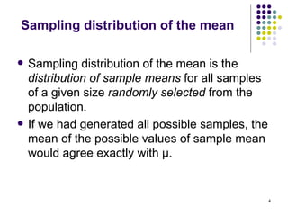
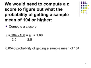
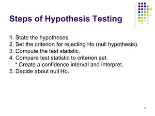
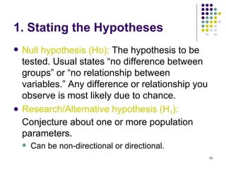
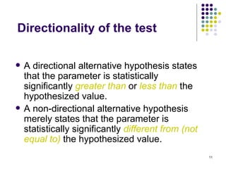
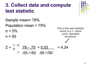
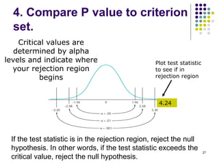
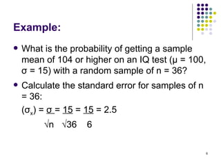
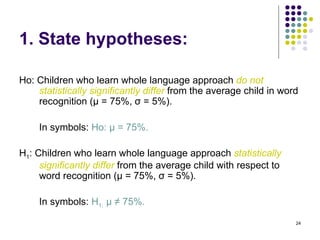
1. The document discusses hypothesis testing using the z-test. It outlines the steps of hypothesis testing including stating hypotheses, setting the criterion, computing test statistics, comparing to the criterion, and making a decision. 2. Examples are provided to demonstrate a non-directional and directional z-test, including stating hypotheses, computing test statistics, comparing to criteria, and interpreting results. 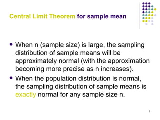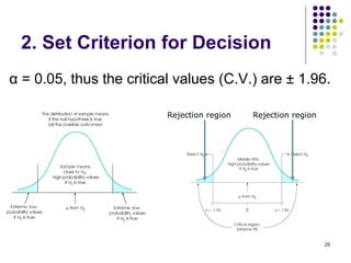3. Key concepts reviewed are the central limit theorem, type I and II errors, significance levels, rejection regions, p-values, and confidence intervals in hypothesis testing.

1. Week 7:
Hypothesis Testing:
z-test
1

2. Review
 We have seen descriptive statistics, statistical
procedures to summarize data and describe
distributions and individual scores.
 We also need inferential statistics, techniques
that can help us to test hypotheses, to
generalize results to a given population, and
to estimate the parameters of a population.
2

3. Statistics and Parameters
 Statistics are the facts on which we draw
conclusions about parameters.
 Sample statistics are only estimates of the
population parameters.
 We need to know how the sample we have
taken compares with other samples that
might be taken from the population.
3

4. Sampling distribution of the mean
 Sampling distribution of the mean is the
distribution of sample means for all samples
of a given size randomly selected from the
population.
 If we had generated all possible samples, the
mean of the possible values of sample mean
would agree exactly with μ.
4

5. Central Limit Theorem for sample mean
 When n (sample size) is large, the sampling
distribution of sample means will be
approximately normal (with the approximation
becoming more precise as n increases).
 When the population distribution is normal,
the sampling distribution of sample means is
exactly normal for any sample size n.
5

6. Example:
 What is the probability of getting a sample
mean of 104 or higher on an IQ test (μ = 100,
σ = 15) with a random sample of n = 36?
 Calculate the standard error for samples of n
= 36:
(σx) = σ = 15 = 15 = 2.5
√n √36 6
6

7. Draw the distribution of the
sample means:
92.5 95 97.5 100 102.5 105 107.5
The probability of getting a sample mean of 107.5 is .0013.
The probability of getting a sample mean of 104 or higher is ____.
7

8. We would need to compute a z
score to figure out what the
probability of getting a sample
mean of 104 or higher:
 Compute a z score:
Z = 104 - 100 = 4 = 1.60
2.5 2.5
0.0548 probability of getting a sample mean of 104.
8

9. Steps of Hypothesis Testing
1. State the hypotheses.
2. Set the criterion for rejecting Ho (null hypothesis).
3. Compute the test statistic.
4. Compare test statistic to criterion set.
* Create a confidence interval and interpret.
5. Decide about null Ho.
9

10. 1. Stating the Hypotheses
 Null hypothesis (Ho): The hypothesis to be
tested. Usual states “no difference between
groups” or “no relationship between
variables.” Any difference or relationship you
observe is most likely due to chance.
 Research/Alternative hypothesis (H1):
Conjecture about one or more population
parameters.
 Can be non-directional or directional.
10

11. Directionality of the test
 A directional alternative hypothesis states
that the parameter is statistically
significantly greater than or less than the
hypothesized value.
 A non-directional alternative hypothesis
merely states that the parameter is
statistically significantly different from (not
equal to) the hypothesized value.
11

12. Examples:
 Non-directional hypothesis:
 There is a statistically significant difference in
males and females on math achievement test
scores.
 How can we rephrase this to be a directional
hypothesis?
12

13. Errors in Inferential Statistics
 Type I error: Reject Ho when it’s true.
 Type II error: Fail to reject Ho when it’s false.
 We’ll discuss Type I error and Type II error when
we look at statistical power next week.
13

14. 2. Setting the Criterion for
Rejecting Ho
 Level of significance (α level): the probability of
making a Type I error when testing a null
hypothesis.
 Establish α level before collecting data. Alpha levels:
.10,.05,.01,.001….
 In deciding to reject the hypothesis at one of these
levels, the researcher knows that the decision to
reject the hypothesis may be incorrect 1%, 5%, or
10% of the time, respectively.
14

15. Rejection Region
 The level of significance represents a proportion of area
in a sampling distribution that equals the probability of
rejecting the Ho if it is true.
 Rejection region refers to the area of the sampling
distribution that represents values for the sample means
that are improbable (possible but highly unlikely) if the
Ho is true.
 The critical values of the test statistic are those values in
the sampling distribution that represent the beginning of
the region of rejection.
 The directionality of the test (one-tailed or two tailed)
affects the critical values.
15

16.  See pages 181 – 188 in text for examples
depicting the relationship between the critical
value and rejection region.
16

17. 3. Computing test statistic to
compute P-value
 P value: The probability of obtaining a value of the
test statistic that is as likely or more likely to reject
Ho as the actual observed value of the test
statistic.
 P value Ranges from 0 to 1.
 Answers: If the populations really have the same
mean overall, what is the probability that random
sampling would lead to a difference between
sample means as large (or larger) than you
observed?
 Do we want a large or small p value?
17

18. Interpreting P-value
 “The probability is greater than .05 that the
observed sample mean would have occurred
by chance if the null hypothesis were true” (p.
195).
 The difference between the sample mean and the
hypothesized value of the population is sufficient
(or not sufficient) enough to attribute it to anything
other than sampling error.
18

19. 4. Compare P value to preset threshold value:
Create confidence interval “Interval Estimate”
 Confidence Interval: Provides an indication of how
accurately the sample mean estimates population
mean.
 An interval of possible values for population mean in
place of using just a single value of sample mean.
 Confidence Coefficient = 1-α
 When α=.05, a 95% confidence interval indicates
that 95% of the time in repeated sampling, intervals
calculated will contain the population mean (true
parameter).
19

20. 5. Make Decision about Ho
1. If P value is less than the threshold, state that
you “reject the null hypothesis” and conclude
that the difference is “statistically significant.”
2. If P value is greater than the threshold, state that
you “fail to reject the null hypothesis” and
conclude that the difference is “not statistically
significant.” The difference is within distribution
of sampling fluctuation.
20

21. Revisiting Hypothesis Testing
Steps:
o State hypotheses.
o Set criterion.
o Compute appropriate test statistic to compute the
P value.
o Compare the P value to the preset threshold
value.
o Make decision.
21

22. Z-test
 Determine the magnitude of the difference
between sample mean and population
mean.
 The population mean μ and its standard
deviation σ are known.
22

23. Z-test Example 1: non-
directional
23

24. 1. State hypotheses:
Ho: Children who learn whole language approach do not
statistically significantly differ from the average child in word
recognition (µ = 75%, σ = 5%).
In symbols: Ho: µ = 75%.
H1: Children who learn whole language approach statistically
significantly differ from the average child with respect to
word recognition (µ = 75%, σ = 5%).
In symbols: H1: µ ≠ 75%.
24

25. 2. Set Criterion for Decision
α = 0.05, thus the critical values (C.V.) are ± 1.96.
Rejection region Rejection region
25

26. 3. Collect data and compute
test statistic
Sample mean= 78%
Population mean = 75%
This is the test statistic
σ = 5% which is a z –score
(unit: standard
n = 50 deviation)
x−µ
Z= σ .78 - .75 = 0.03 = 4.24
n .05 /√50 .05 /√50
26

27. 4. Compare P value to criterion
set.
Critical values are
determined by alpha
levels and indicate where Plot test statistic
your rejection region to see if in
begins rejection region
4.24
If the test statistic is in the rejection region, reject the null
hypothesis. In other words, if the test statistic exceeds the 27
critical value, reject the null hypothesis.

28. 5. Make Decision
 We reject the null hypothesis and conclude
that children who learn the whole language
statistically significantly differ from the
average child in word recognition, z = 4.24, p
< .05.
28

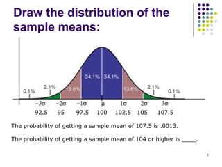
29. Compute confidence interval
 Alpha set a 0.05. Thus, we build a 95% confidence interval and
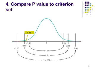
the critical values are ± 1.96.
CI95 = μ ± Critical value (σ ) Standard error
√n
CI95% = .75 ± 1.96 (.05 / √50 ) = .75 ± .01 =
[.74, .76]
 95% of all possible means for samples of size 50 in the population
will fall between 74% and 76%.
 Our sample mean of 78% falls outside of the interval we built.
29

30. Z-test Example 2: Directional
30

31. 1. State hypotheses:
Ho: Babies born to mothers who smoke do not
significantly differ in birth weight than the
average baby (µ = 7.5, σ = 1.2).
Ho: µ = 7.5
H1: Babies born to mothers who smoke weigh
significantly less than the average baby at
birth (µ = 7.5, σ = 1.2).
H1: µ < 7.5.
31

32. 2. Set Criterion.
α = 0.05
 Since this is a directional test, only look at
one side (tail) of the distribution.
 What is the z-score corresponding to 0.05?
 1.64 + 1.65 / 2 = 1.645.
 Use - 1.645 since the hypothesized mean is
smaller than the population mean in the H1.
32

33. 3. Compute Test Statistic.
Sample mean = 7.1
Population mean = 7.5
σ = 1.2 This is the test statistic
which is a z –score
(unit: standard
n = 50 deviation)
x−µ
Z= = 7.1 – 7.5 = -.40 = -2.36
σ 1.2 /√50 1.2 /√50
n
33

34. 4. Compare P value to criterion
set.
-2.36
34

35. 5. Make Decision.
We reject the null hypothesis and conclude
that babies born to mothers who smoke
weigh statistically significantly less than the
average baby at birth, z = -2.36, p < .05.
35

36. Compute confidence interval:
CI95 = μ ± Critical value (σ )
√n
CI95 = 7.5 - 1.645 (1.2) = 7.22
√50
 Directional test: Any group of 50 babies born to
mothers who smoke who are less than 7.22
pounds are significantly lower than the
average baby.
36

37. Recommended note cards:
 Steps in hypothesis testing
 Critical values associated with alpha levels of .05
and .01 (most commonly used) for a one and two-
tailed test. Use page 189 in your text as a guide.
 Z-test
 When to use a Z-test
 Formula for computing a Z-test
 Confidence interval
 Formula
 Interpretation
37