Downloaded 144 times
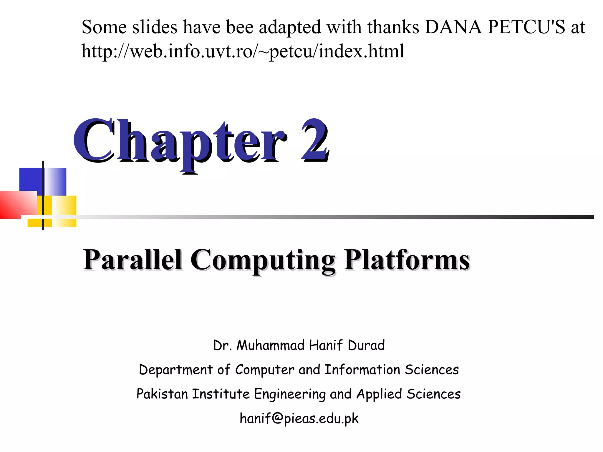

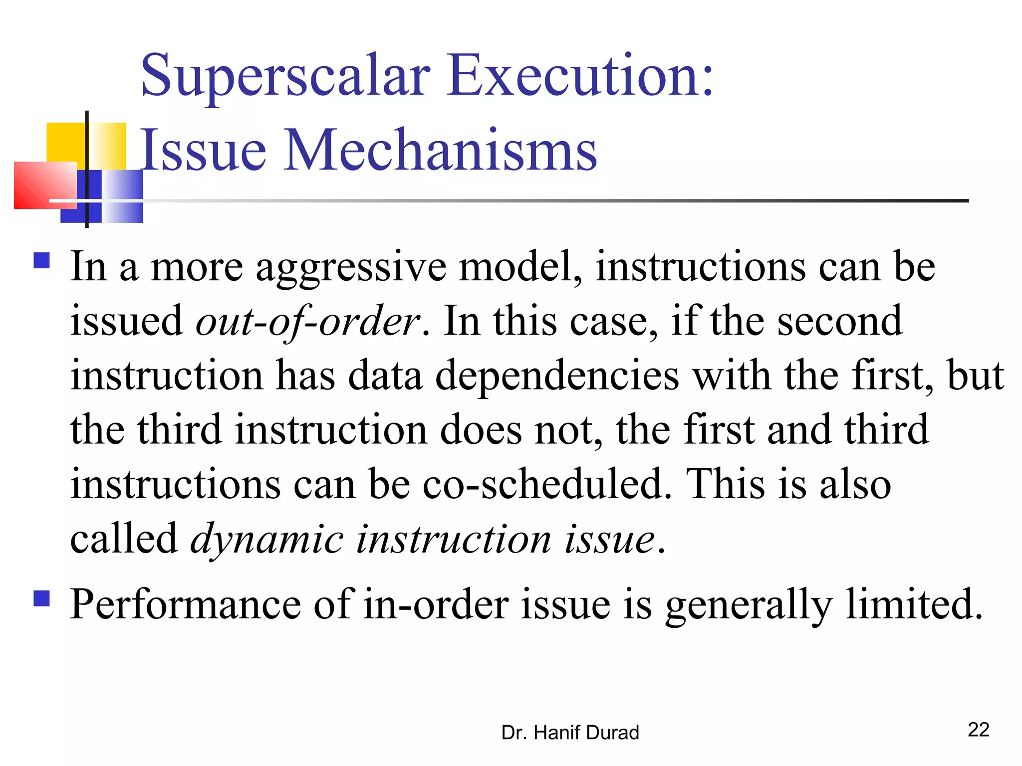

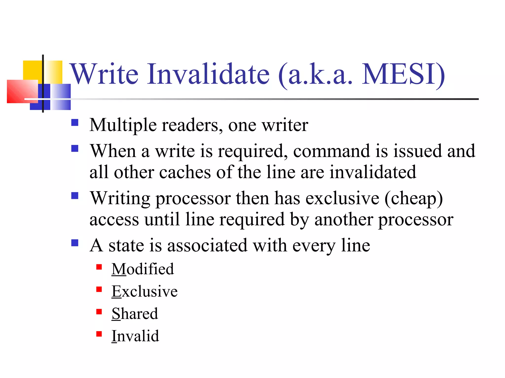
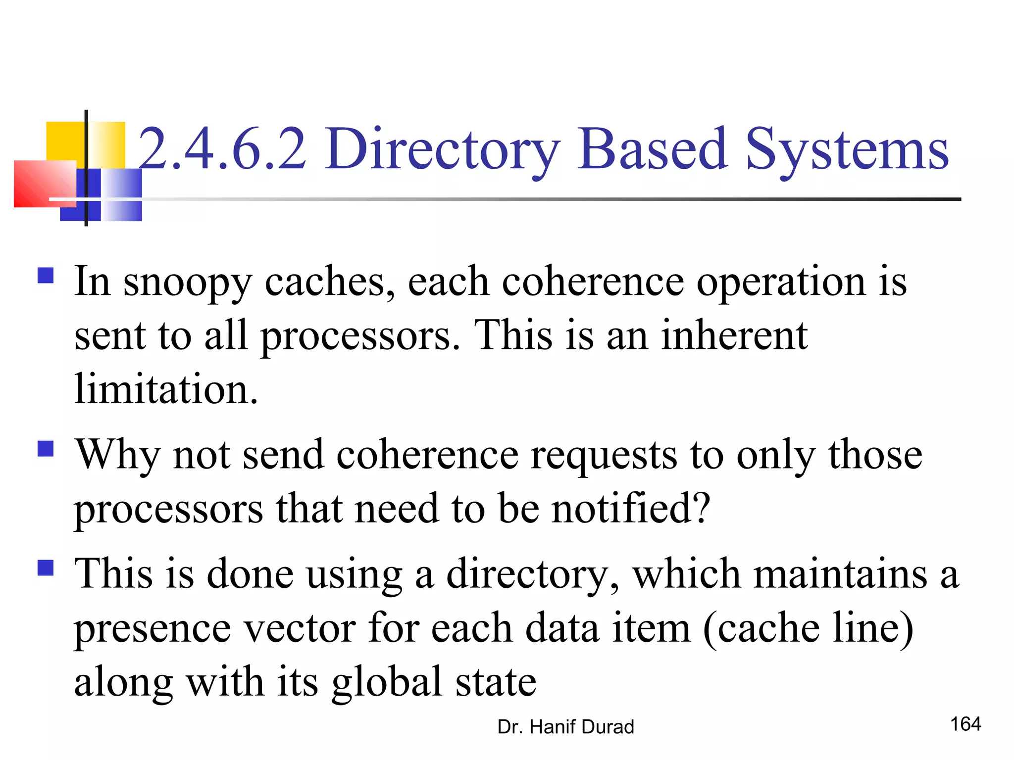
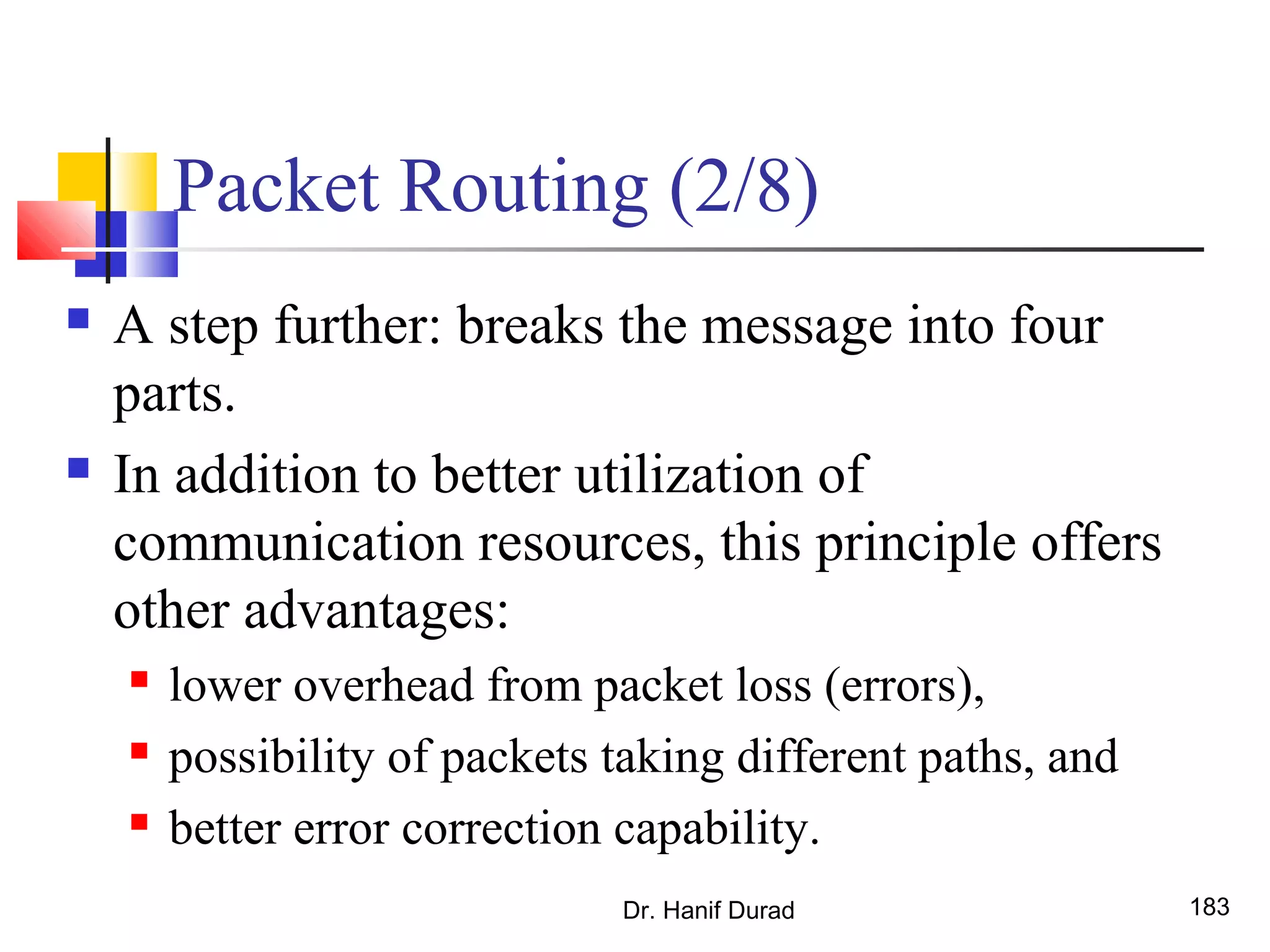
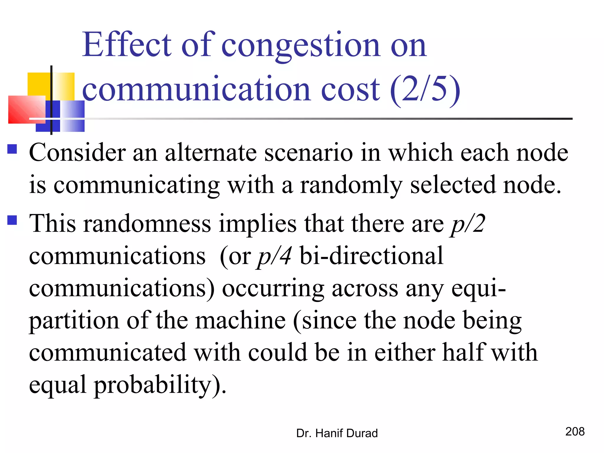
![Example 2.5 Impact of Strided Access
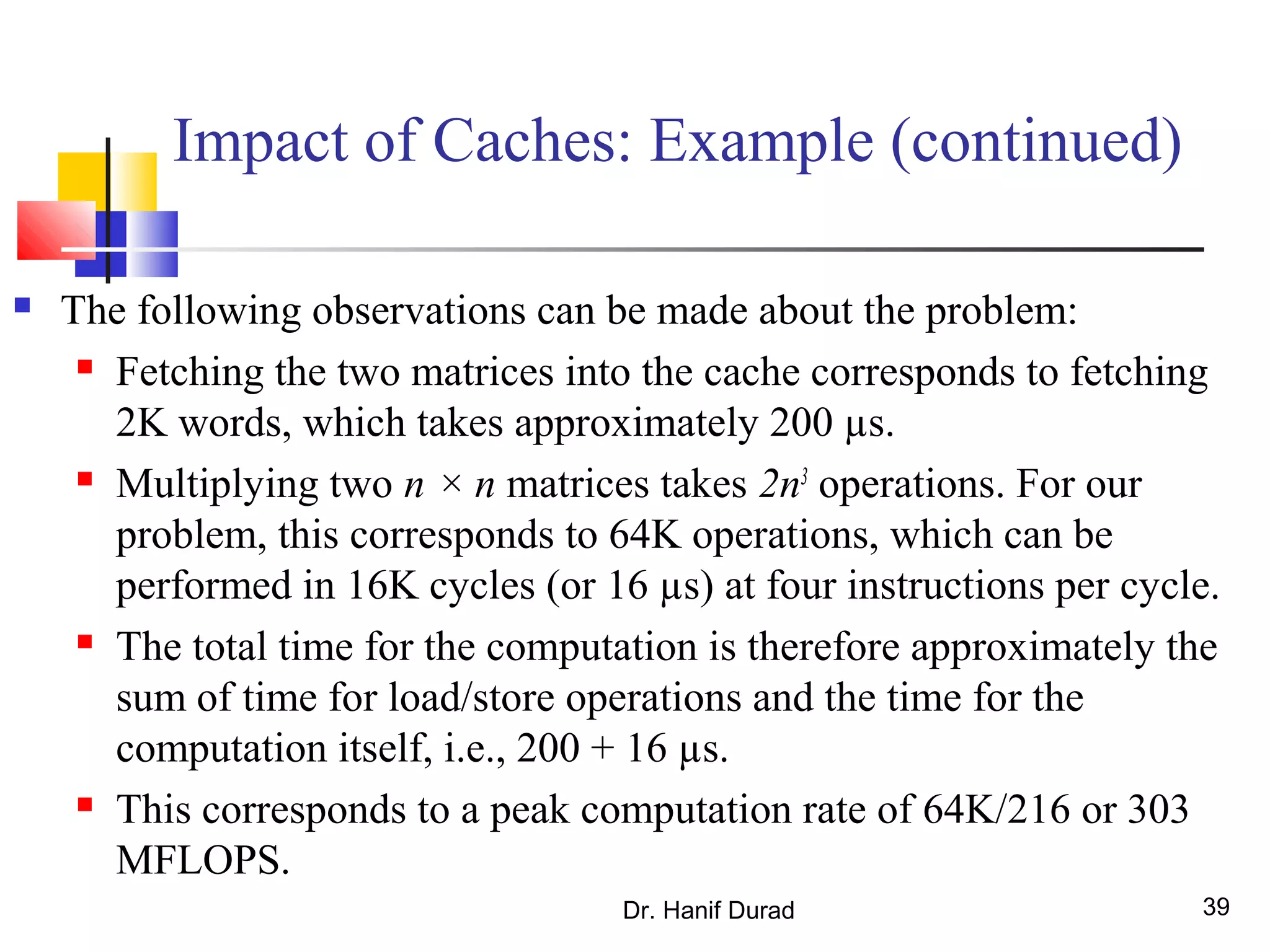
Consider the following code fragment:
for (i = 0; i < 1000; i++)
b[i] = 0.0;
for (j = 0; j < 1000; j++)
b[i] += A[j][i];
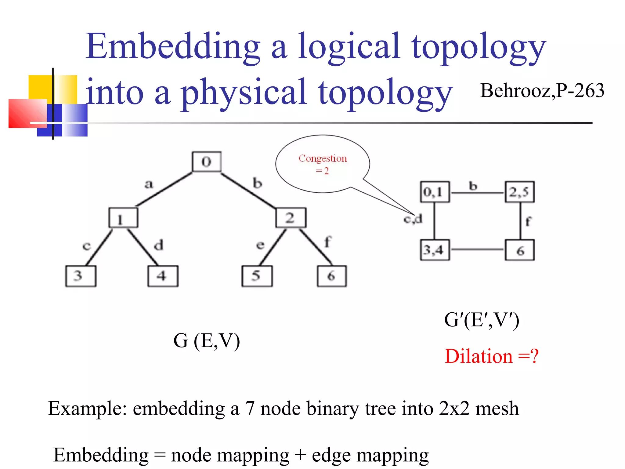
The code fragment sums columns of the matrix A
into a vector b.
Dr. Hanif Durad 46](https://image.slidesharecdn.com/chapter2pc-150609040909-lva1-app6891/75/Chapter-2-pc-46-2048.jpg)
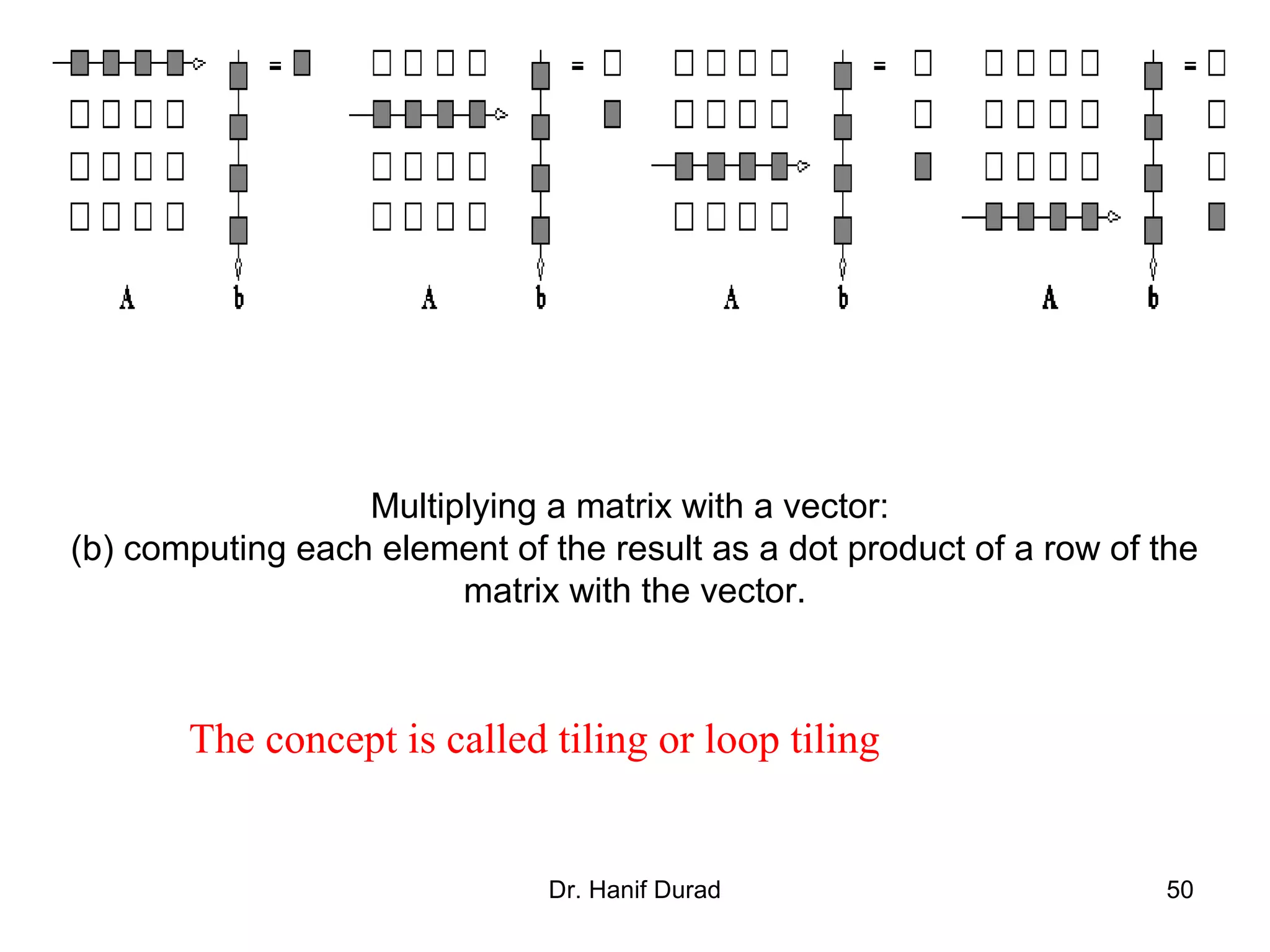
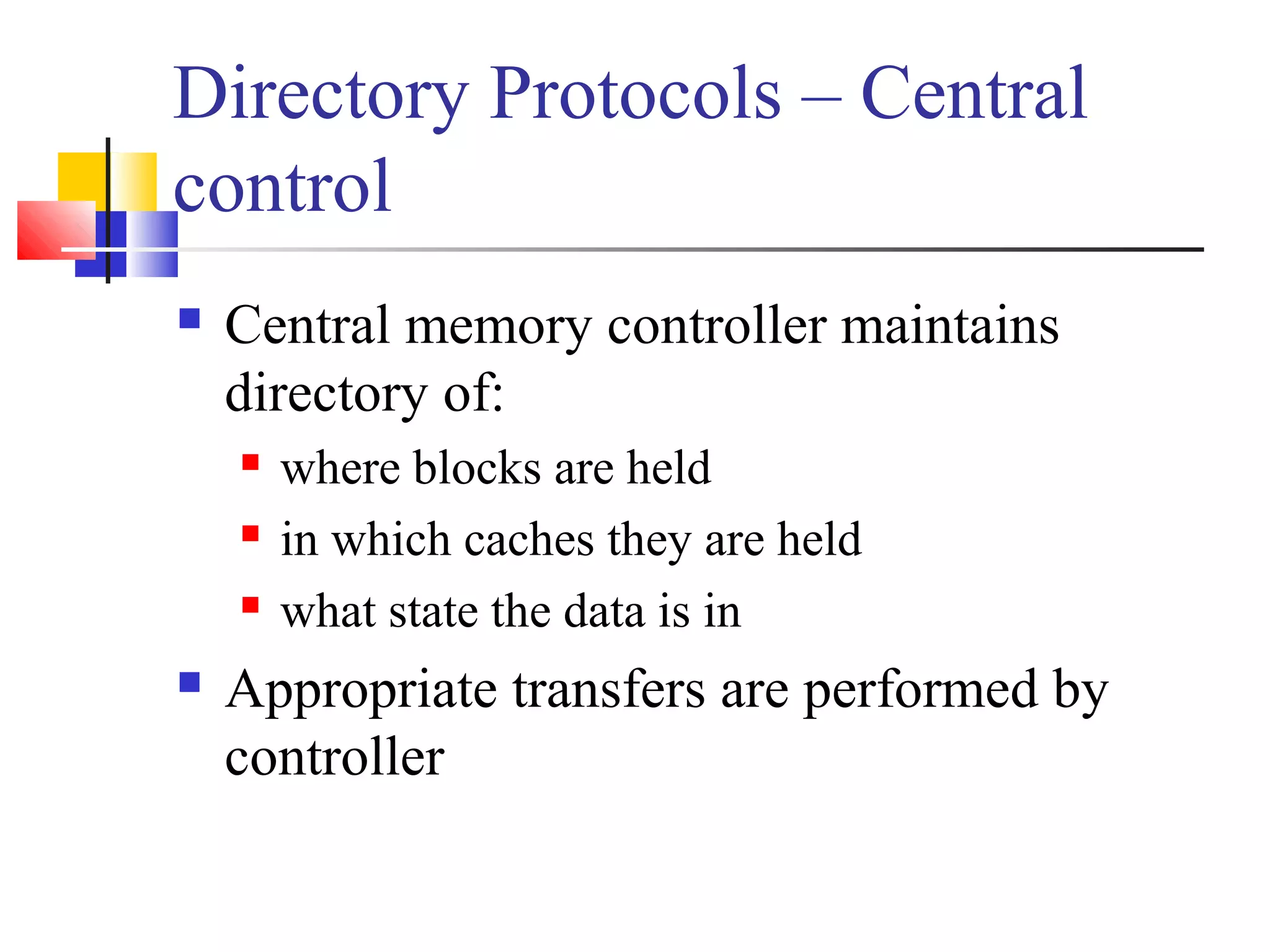
![Dr. Hanif Durad 49
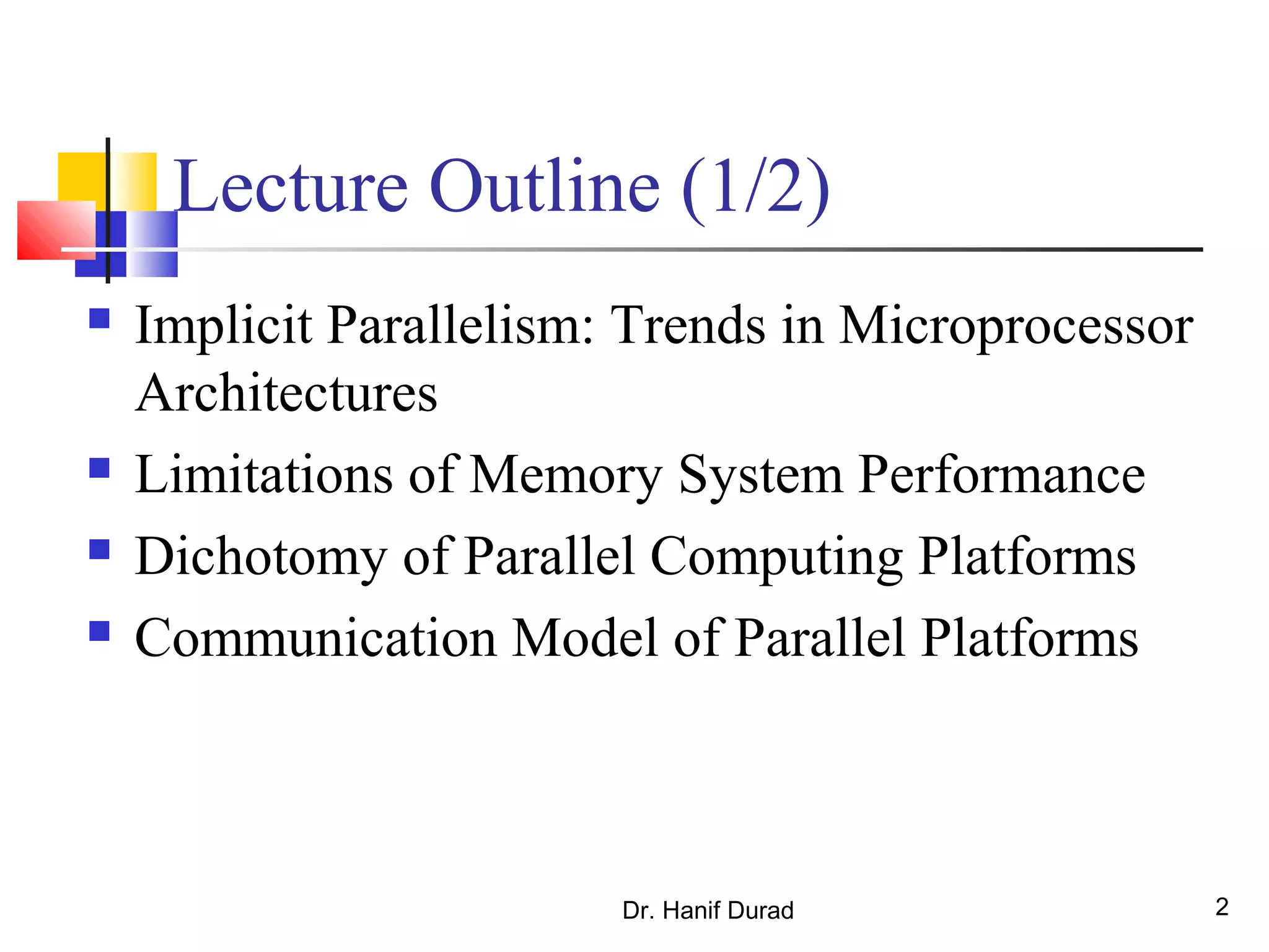
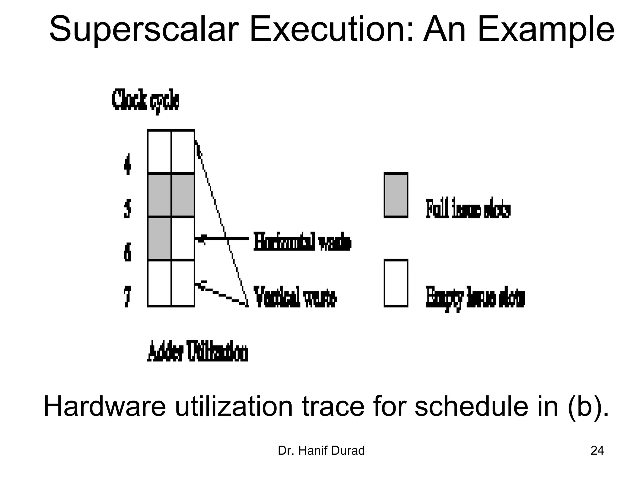
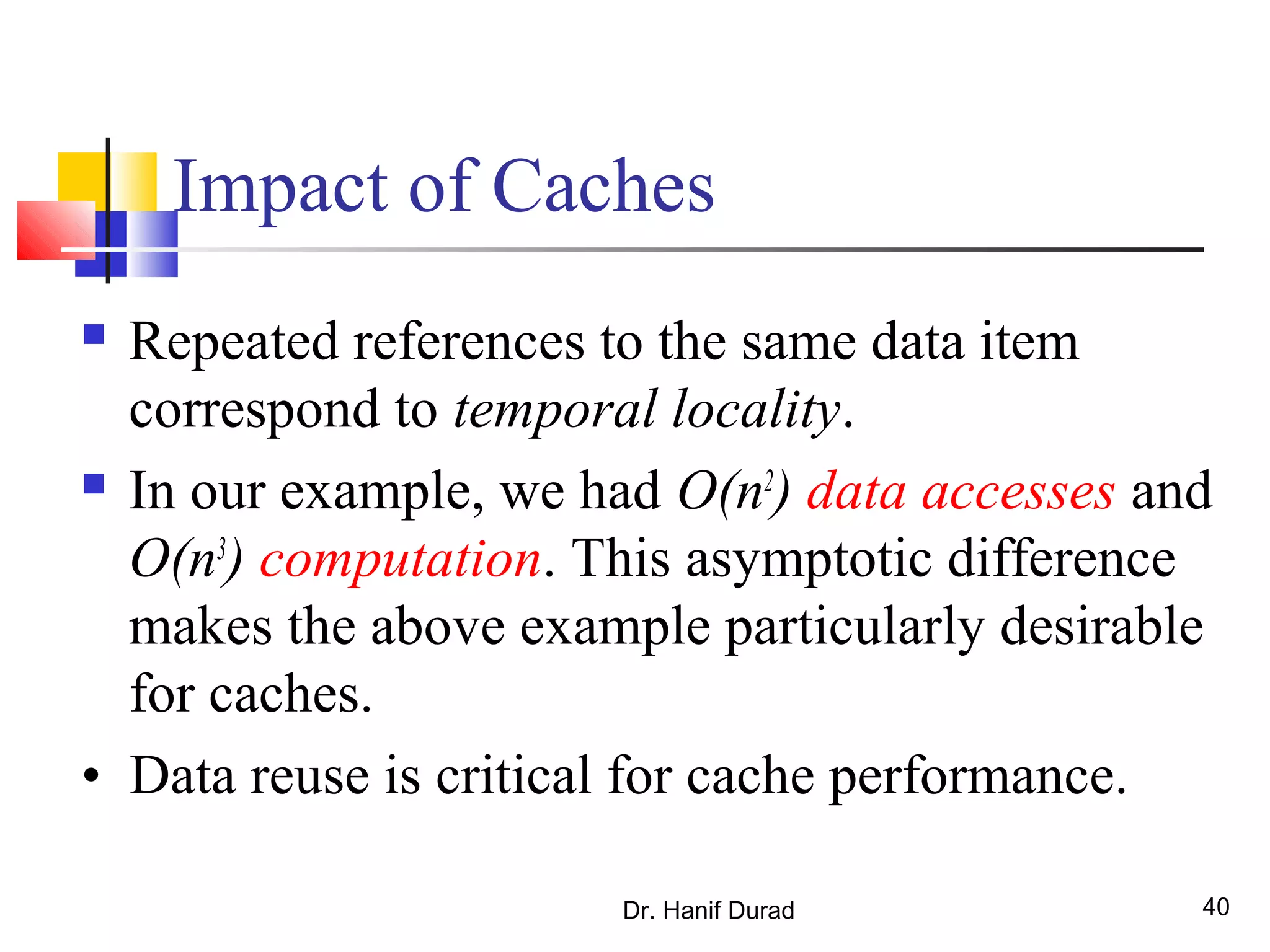
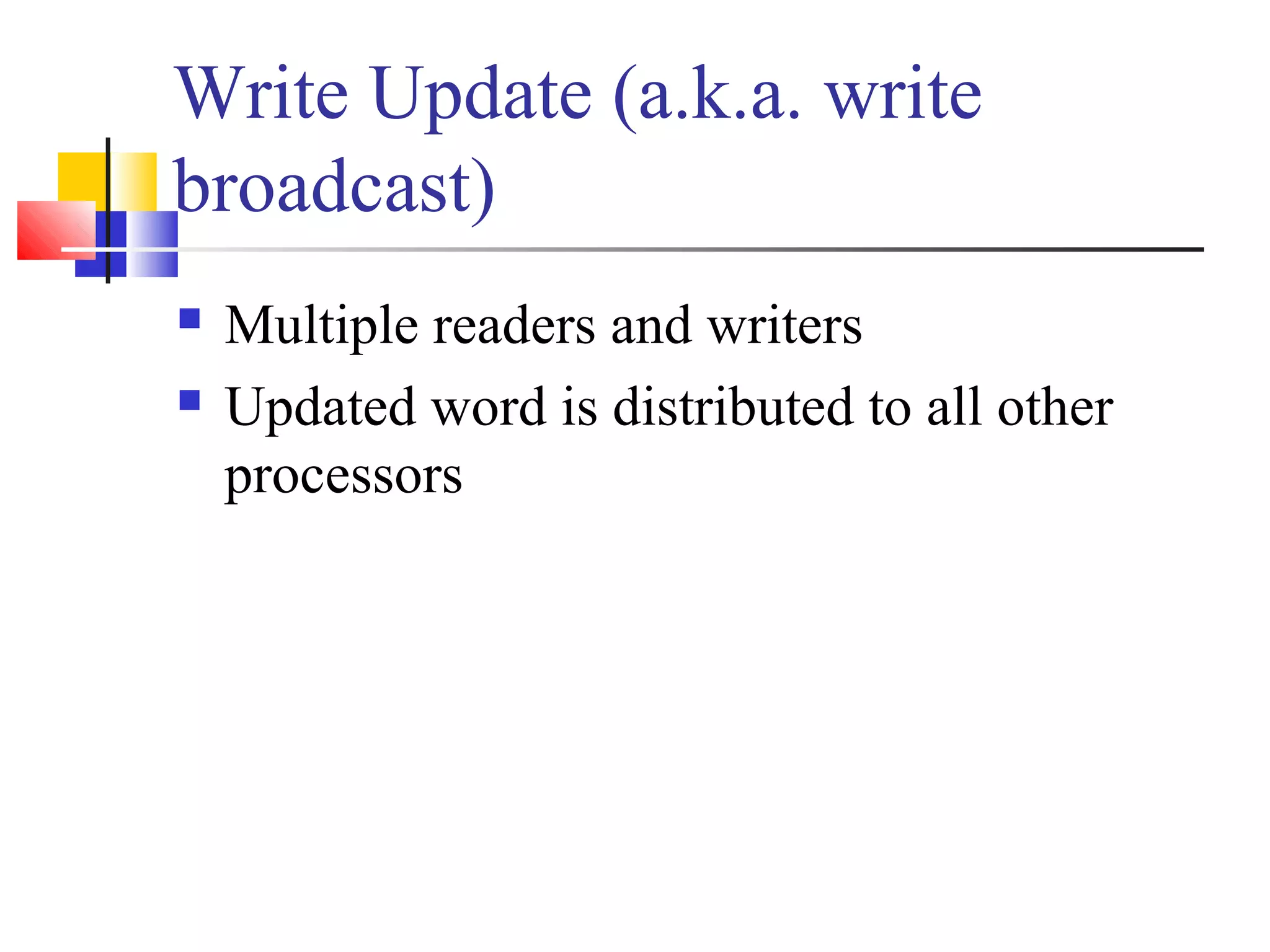
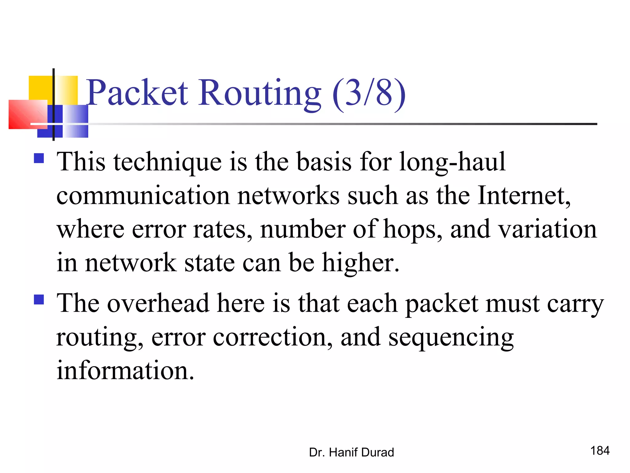
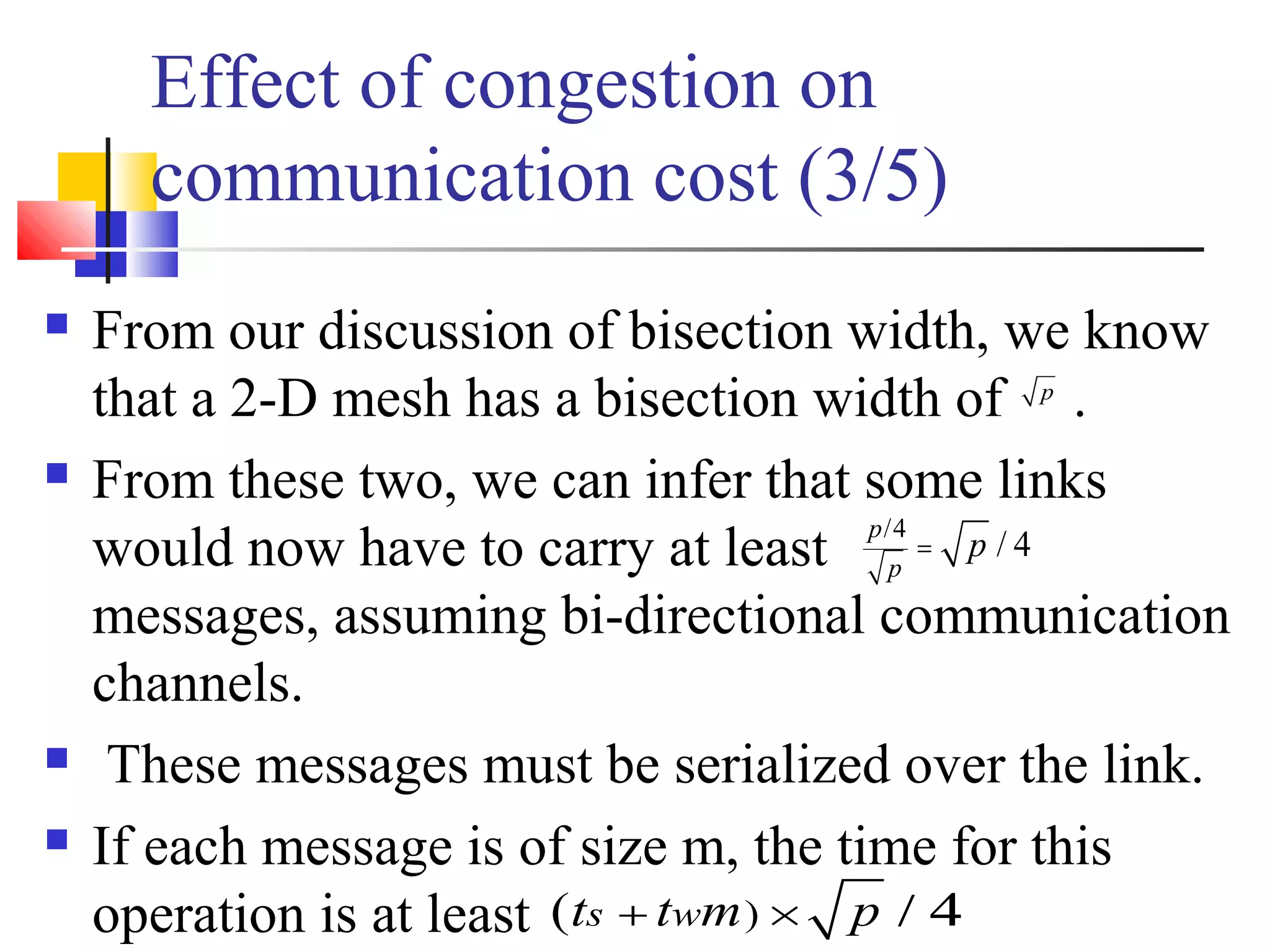
Example 2.6 Eliminating Strided Access
We can fix the above code as follows:
for (i = 0; i < 1000; i++)
b[i] = 0.0;
for (j = 0; j < 1000; j++)
for (i = 0; i < 1000; i++)
b[i] += A[j][i];
In this case, the matrix is traversed in a row-order and performance
can be expected to be significantly better.](https://image.slidesharecdn.com/chapter2pc-150609040909-lva1-app6891/75/Chapter-2-pc-49-2048.jpg)
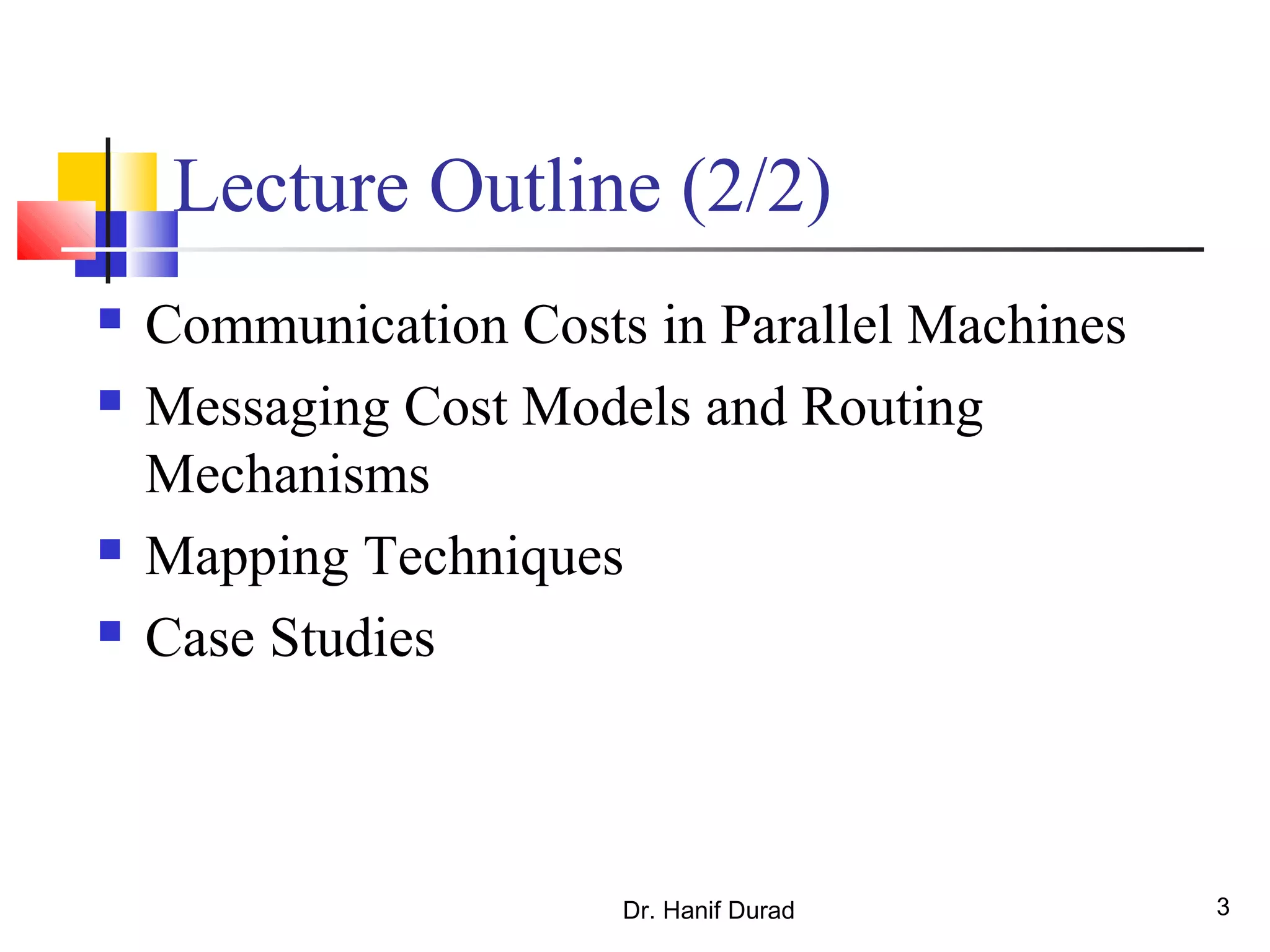
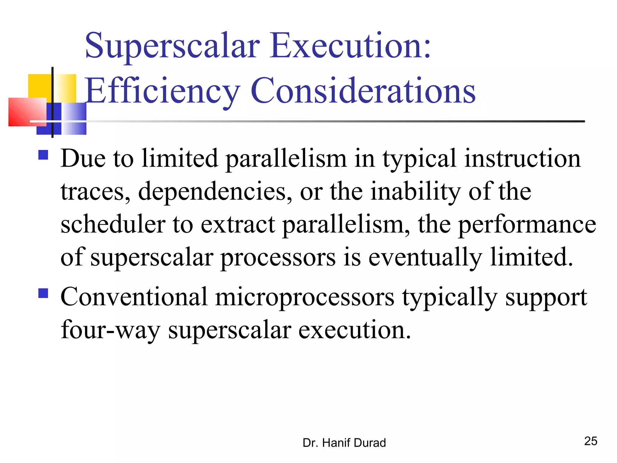
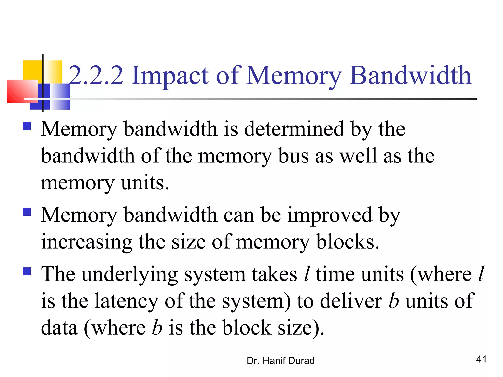
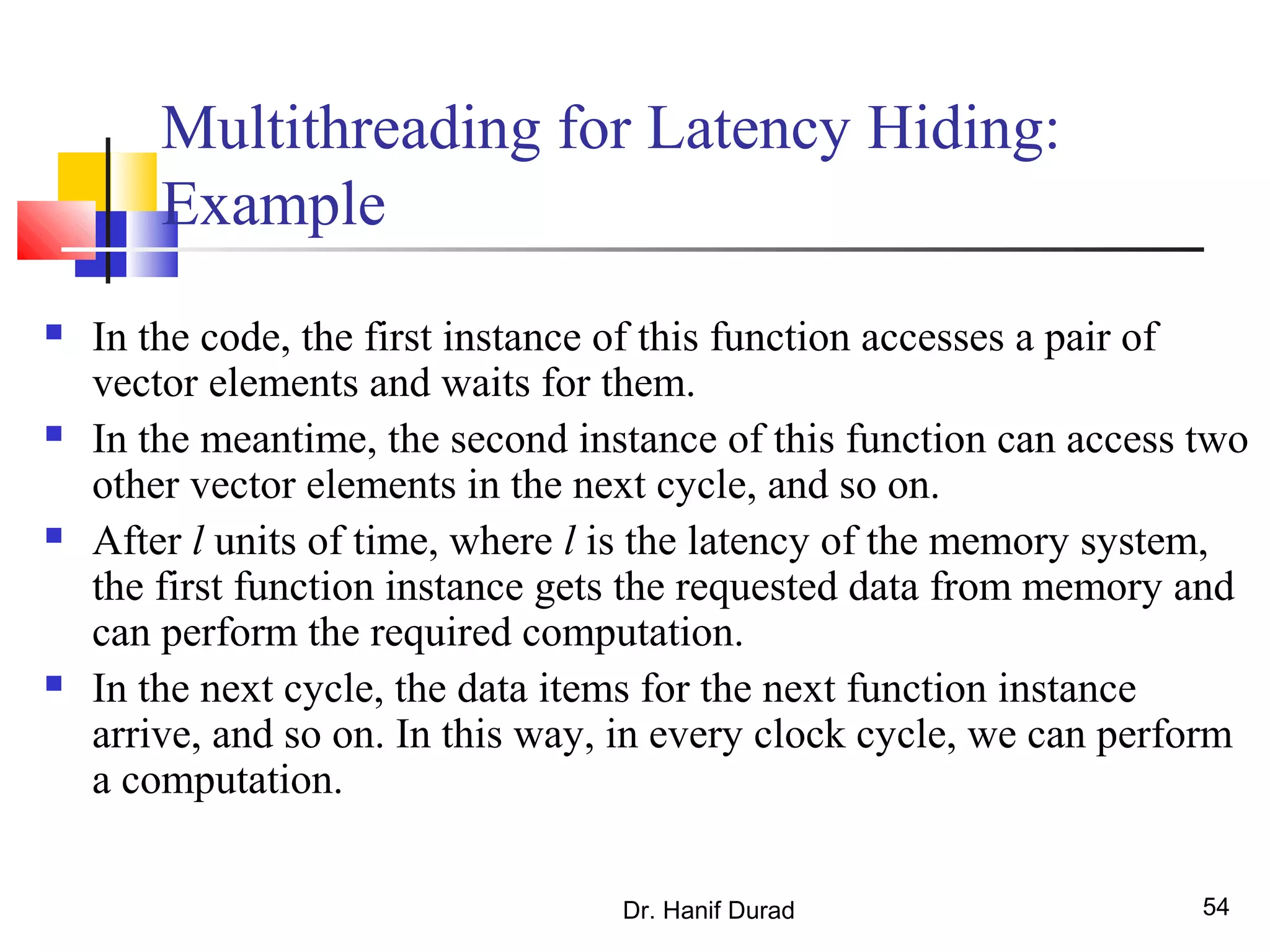
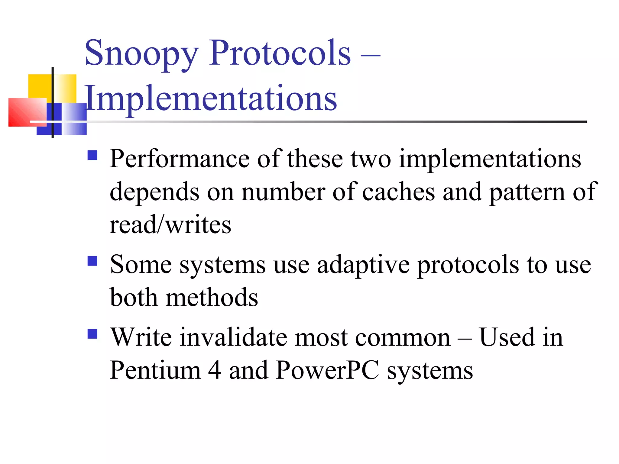
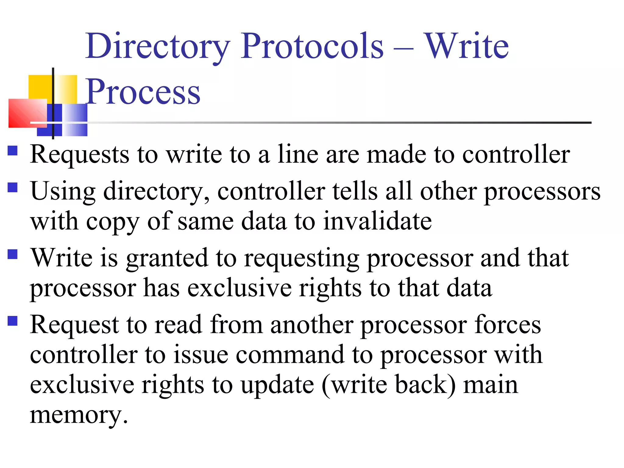
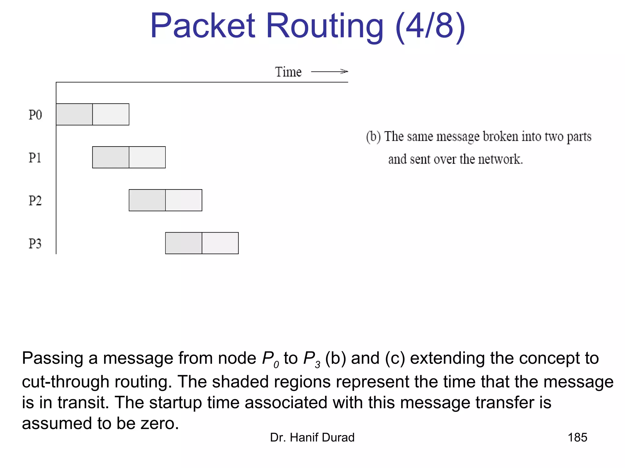
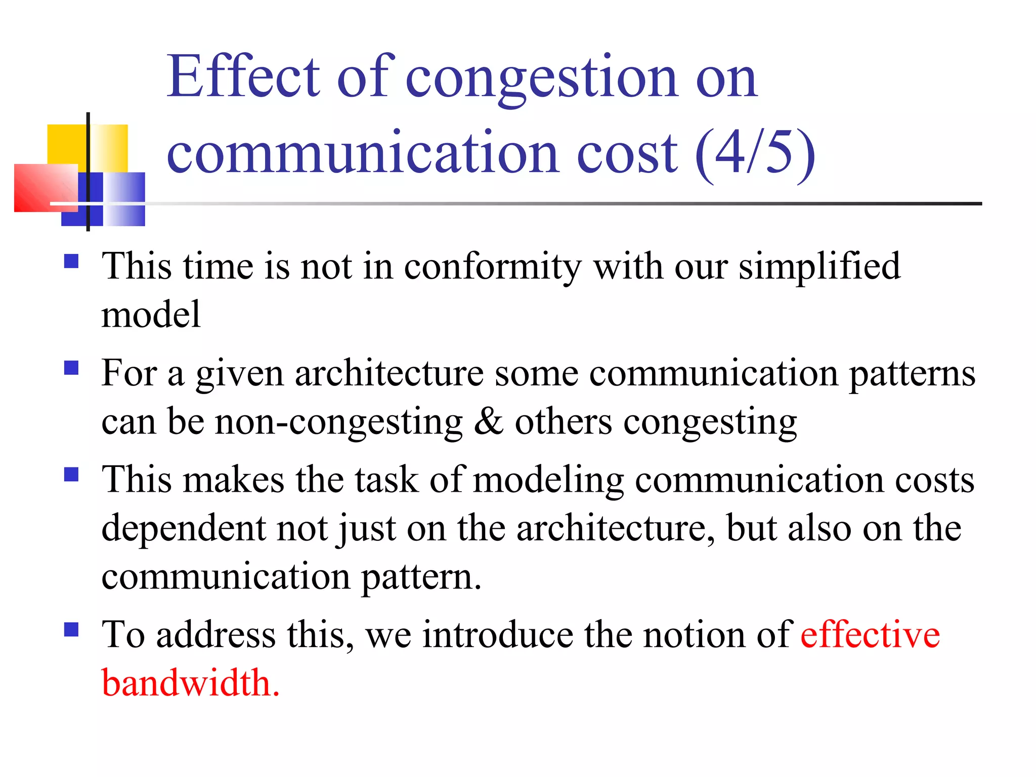
![2.2.3.1 Multithreading for Latency Hiding
A thread is a single stream of control in the flow of a
program.
We illustrate threads with a simple example:
for (i = 0; i < n; i++)
c[i] = dot_product(get_row(a, i), b);
Each dot-product is independent of the other, and
therefore represents a concurrent unit of execution.
We can safely rewrite the above code segment as:
for (i = 0; i < n; i++)
c[i] = create_thread(dot_product,get_row(a, i),
b);
Example 2.7 Threaded execution of matrix multiplication](https://image.slidesharecdn.com/chapter2pc-150609040909-lva1-app6891/75/Chapter-2-pc-53-2048.jpg)
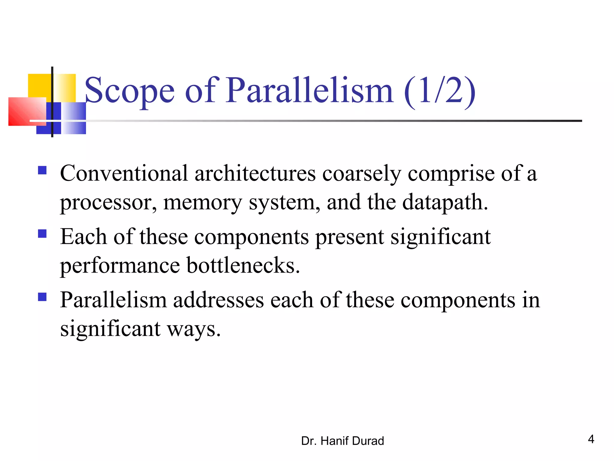
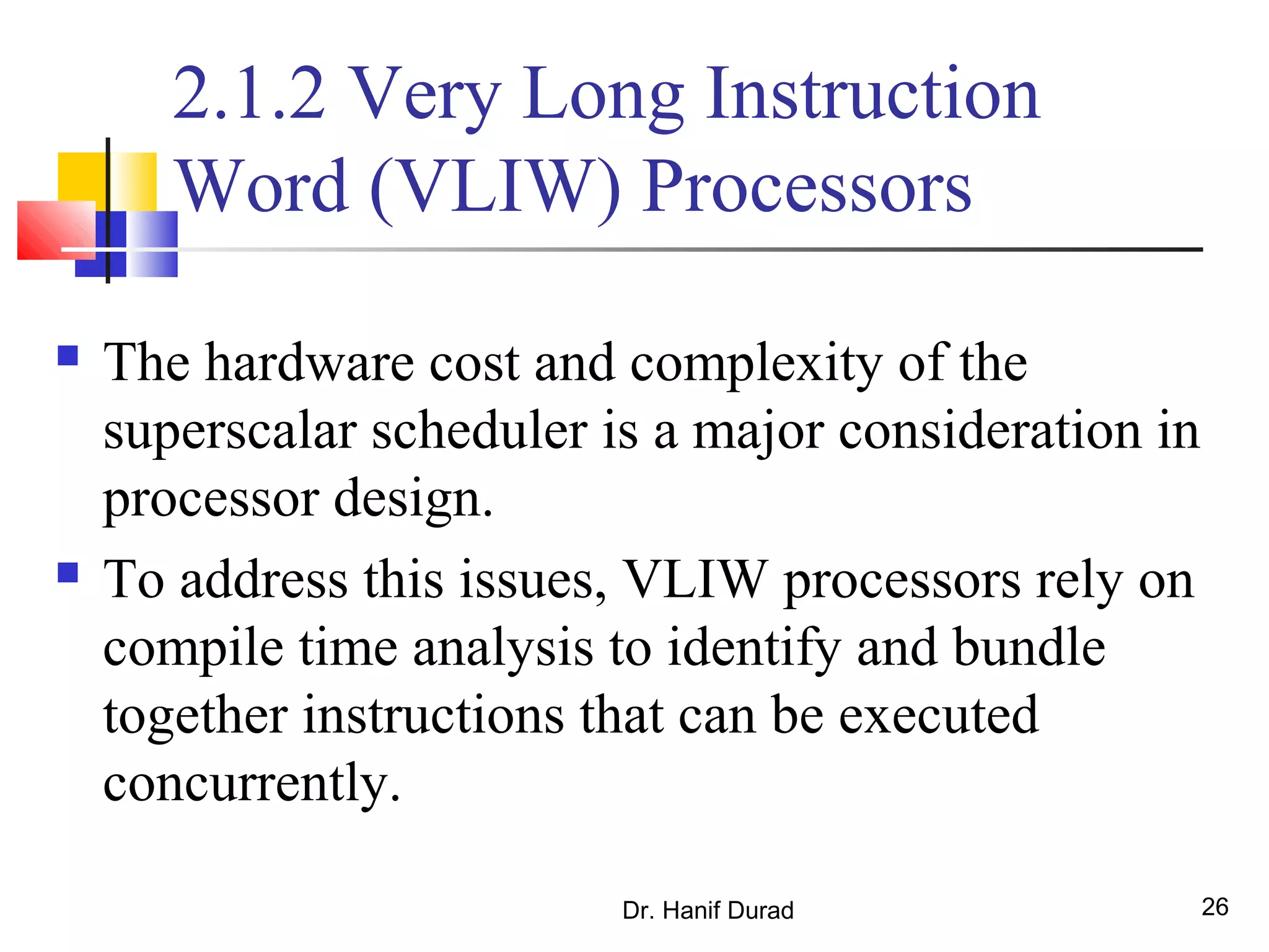
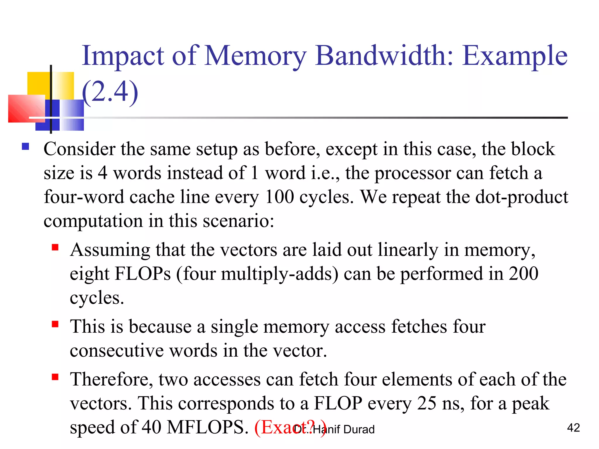
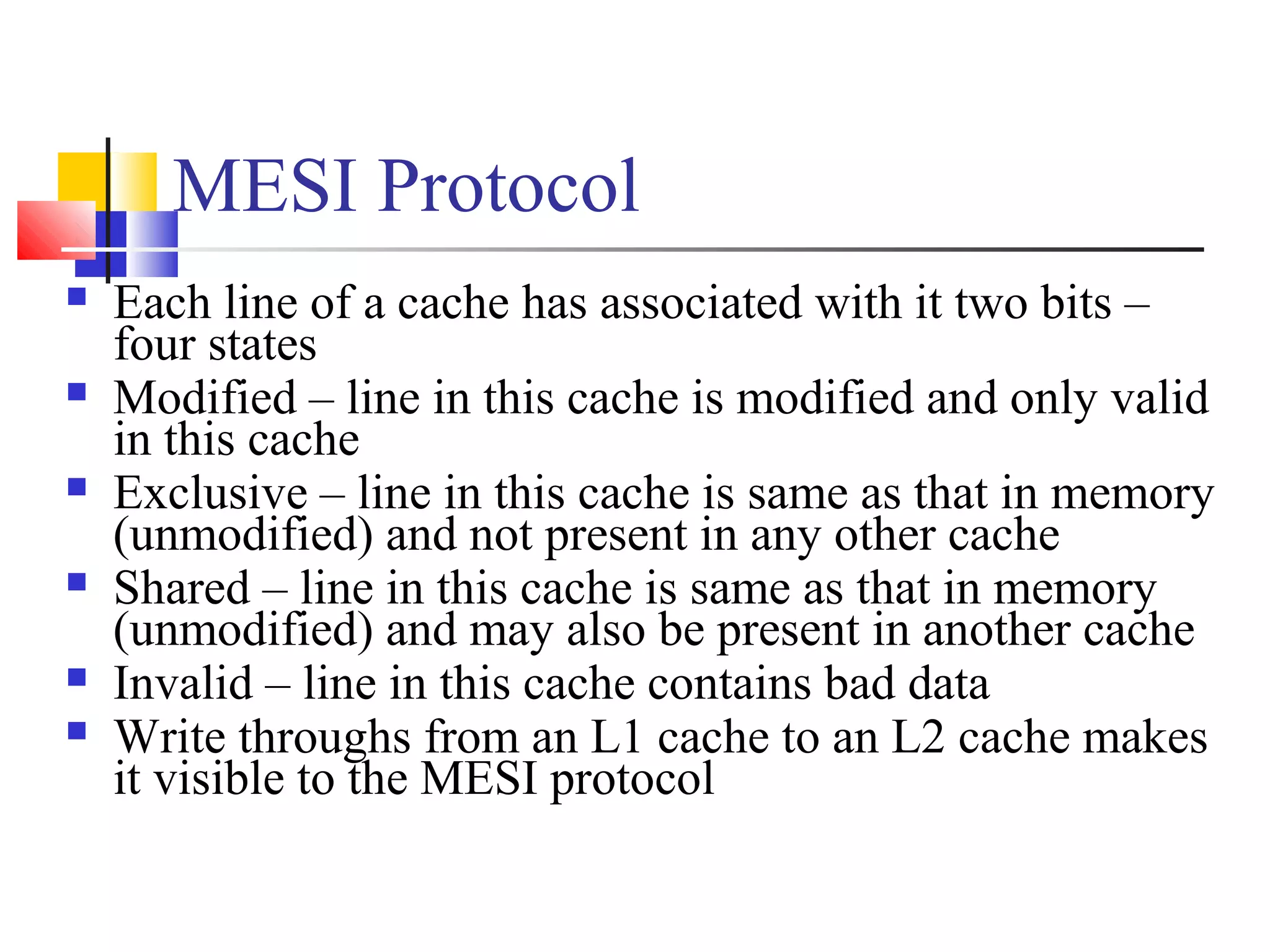
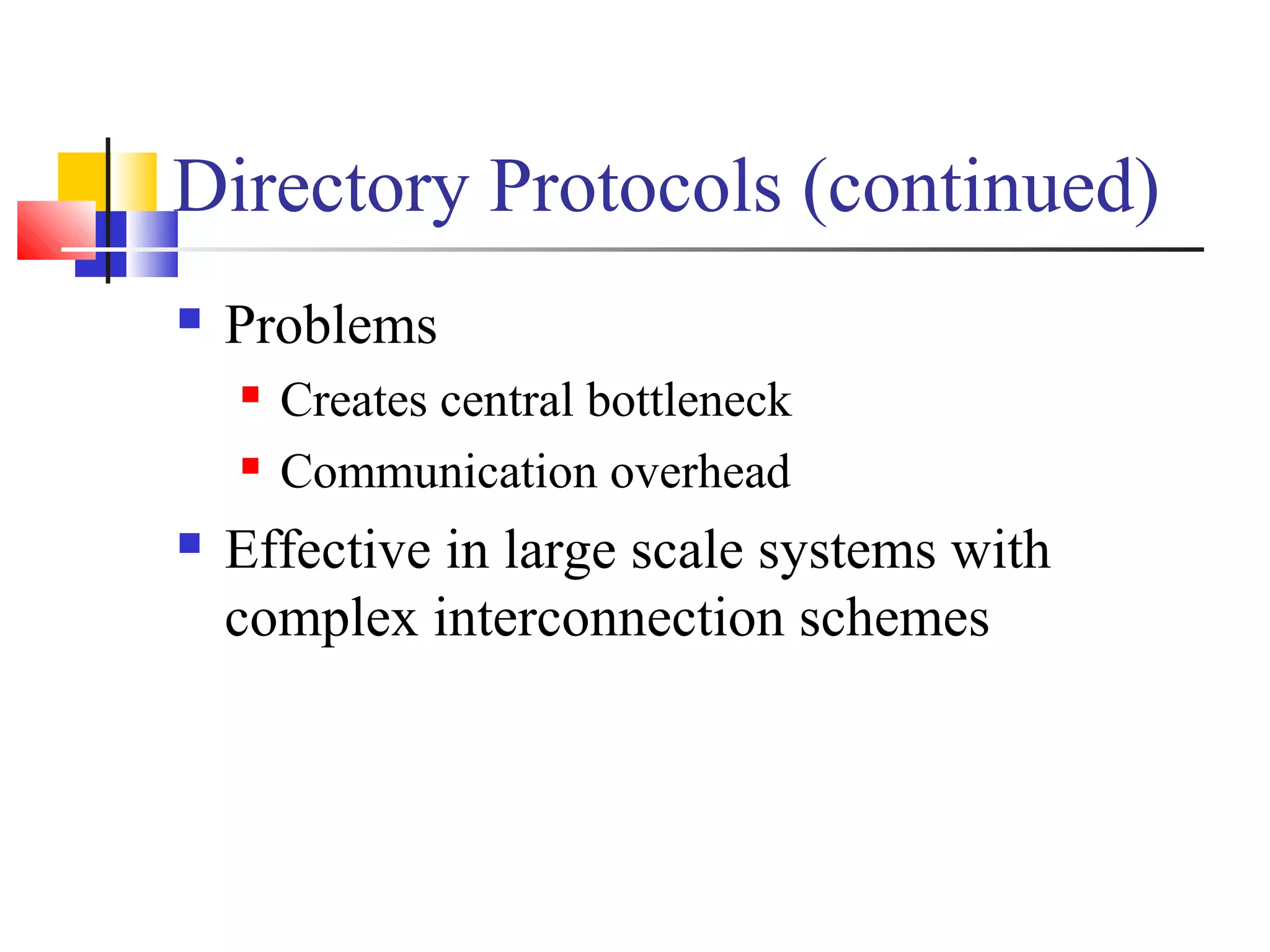
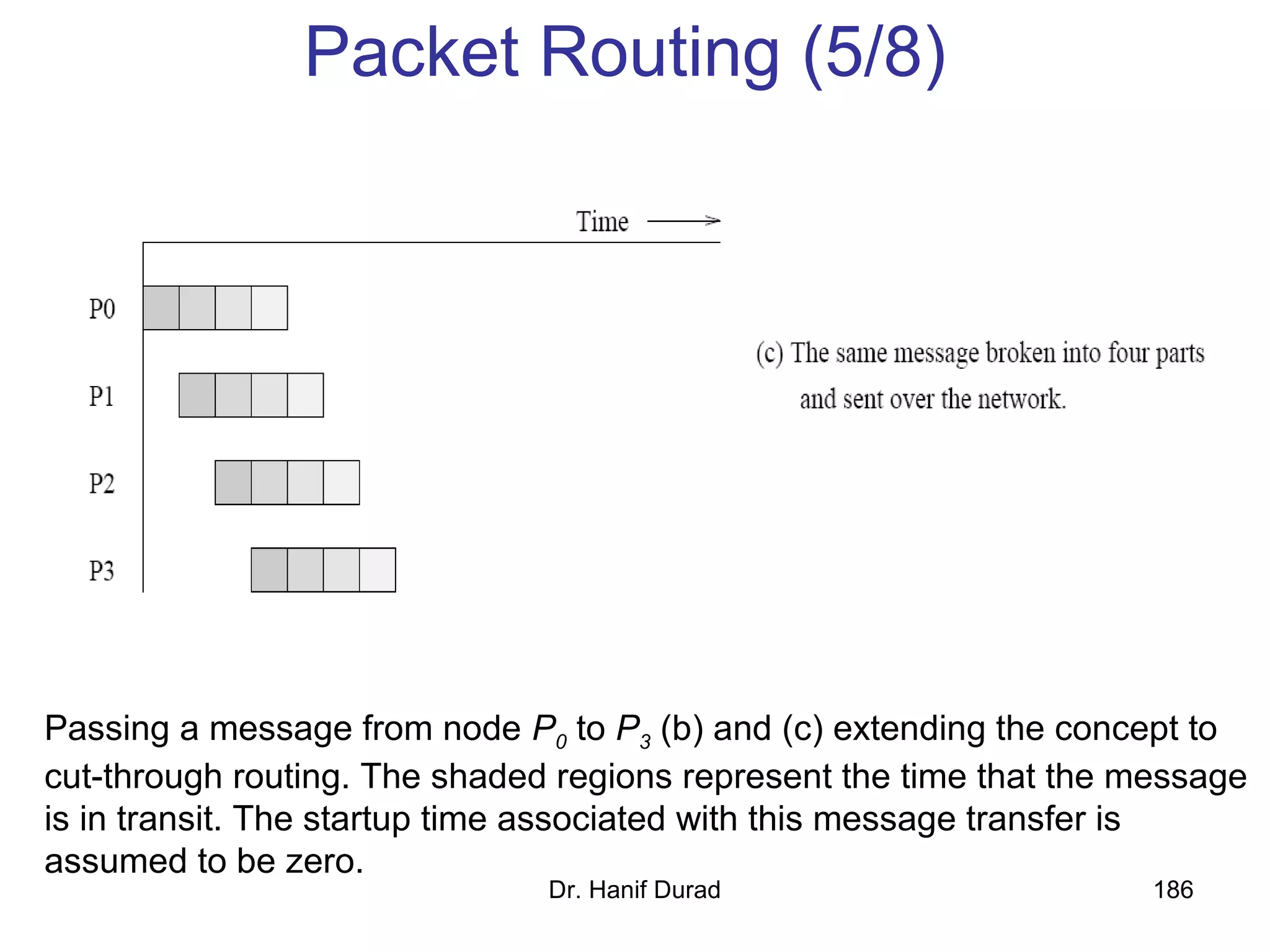
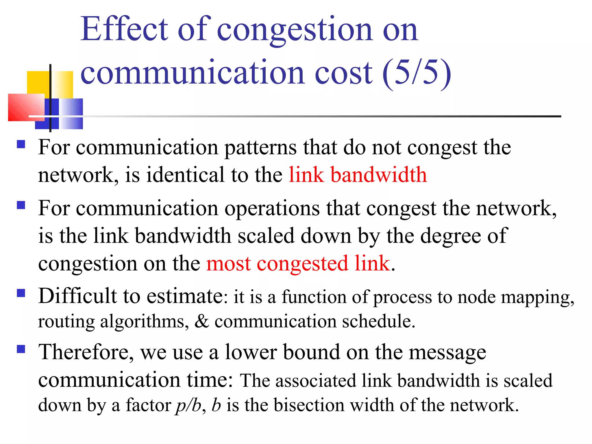
![Example 2.10 Parallelism from single
instruction on multiple processors
Consider the following code segment that
adds two vectors:
for (i = 0; i < 1000; i++)
c[i] = a[i] + b[i];
various iterations of the loop are independent
of each other; can all be executed
independently on all the processors with
appropriate data
we could execute this loop much fasterDr. Hanif Durad 61](https://image.slidesharecdn.com/chapter2pc-150609040909-lva1-app6891/75/Chapter-2-pc-61-2048.jpg)


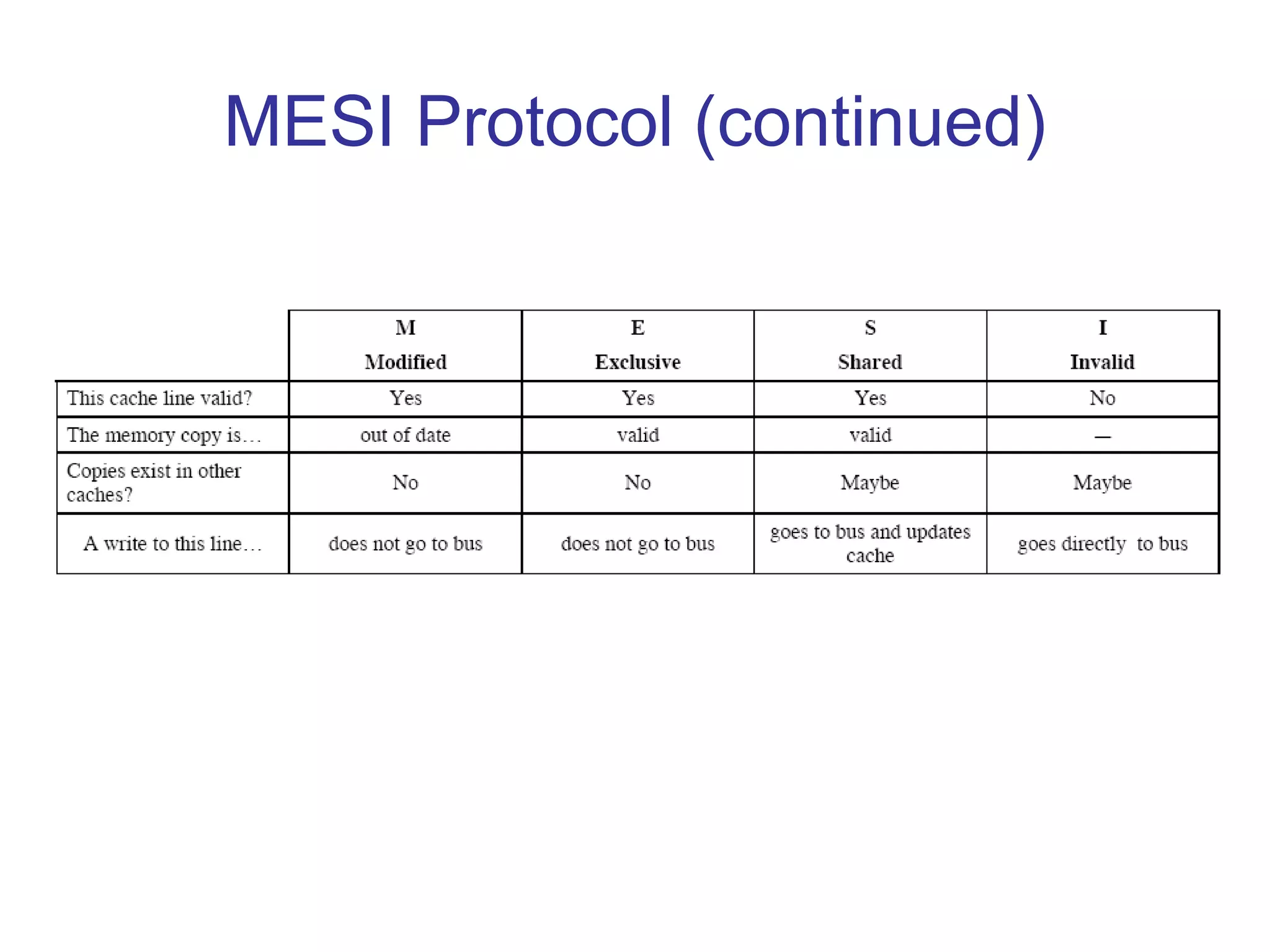
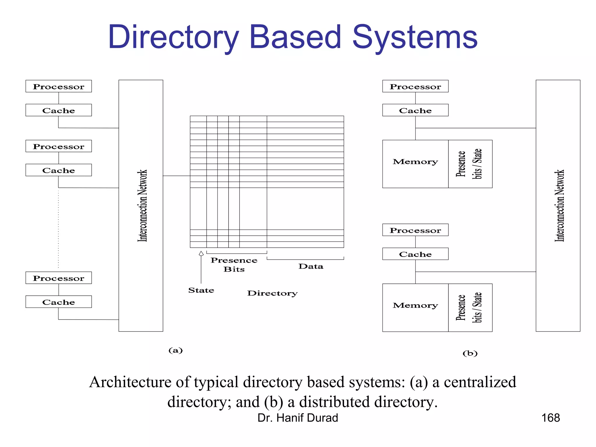


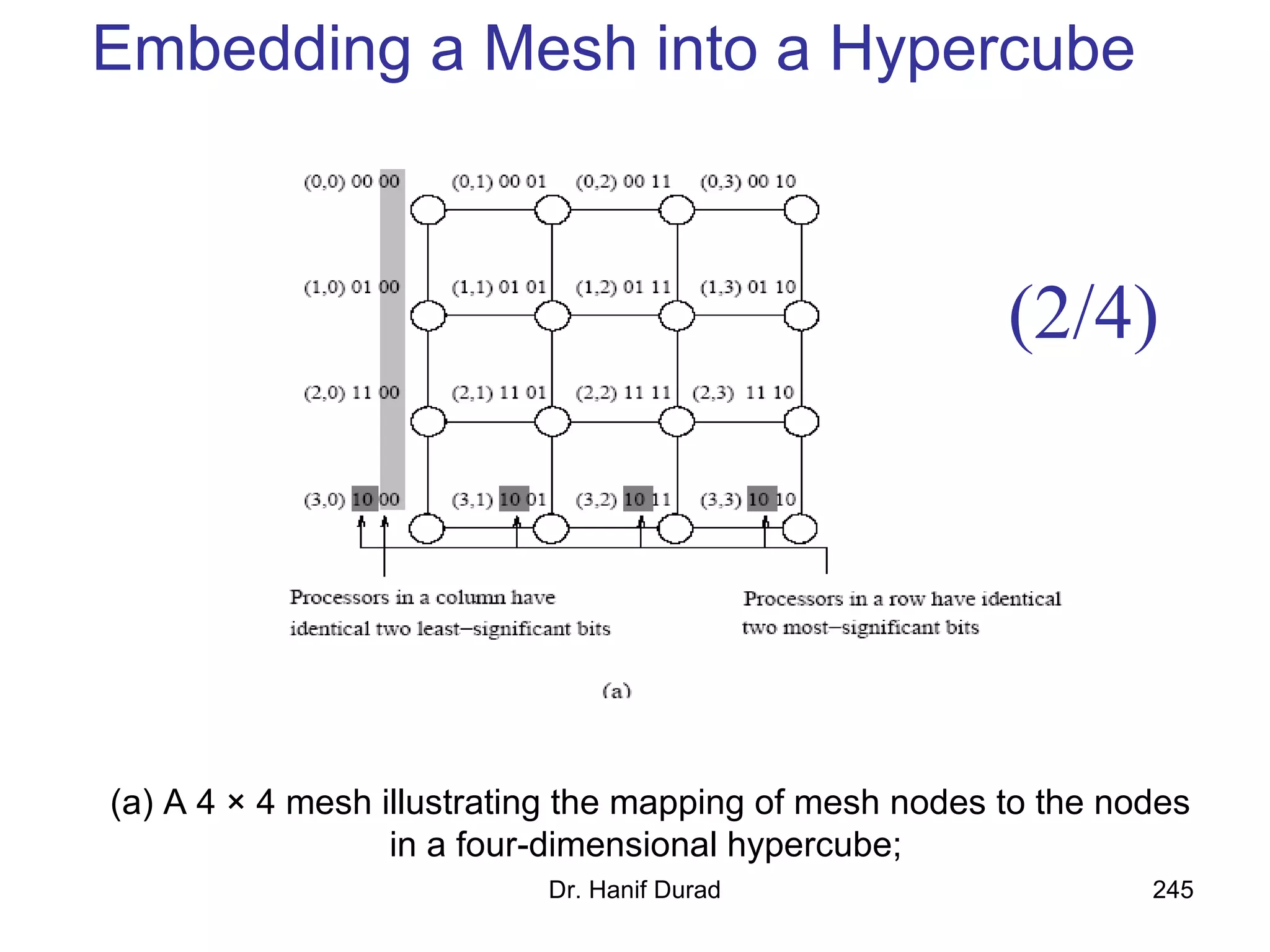
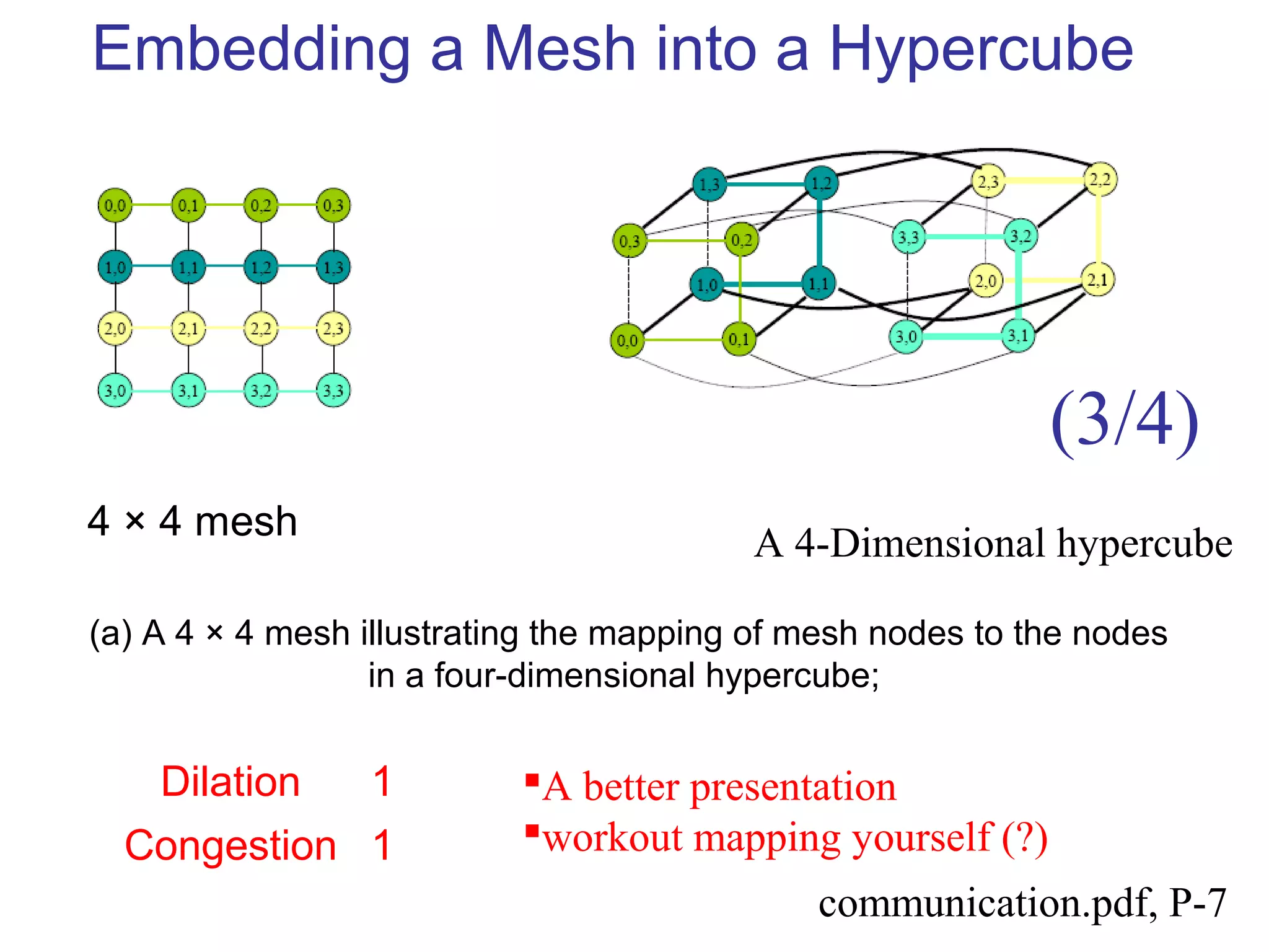
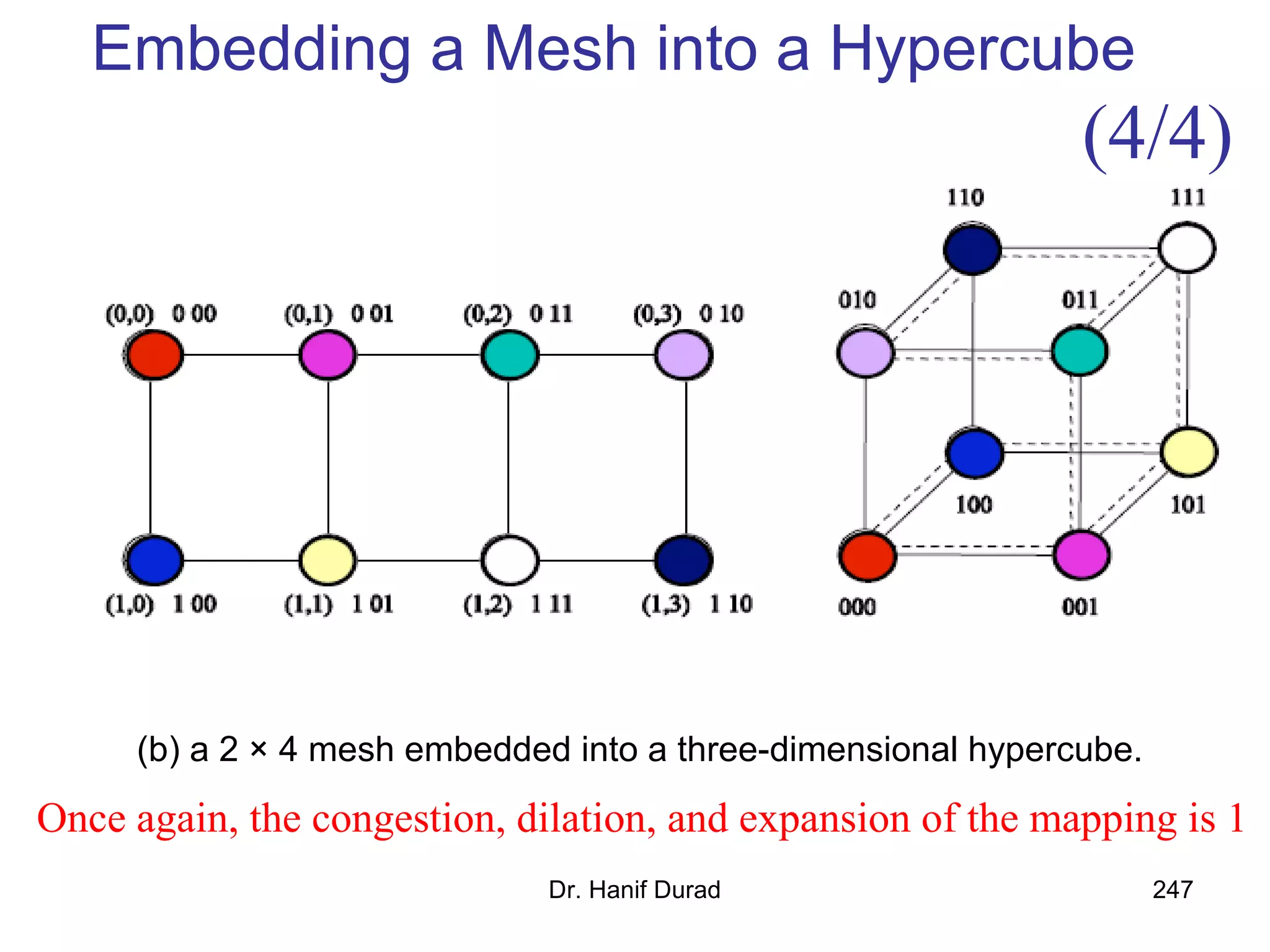

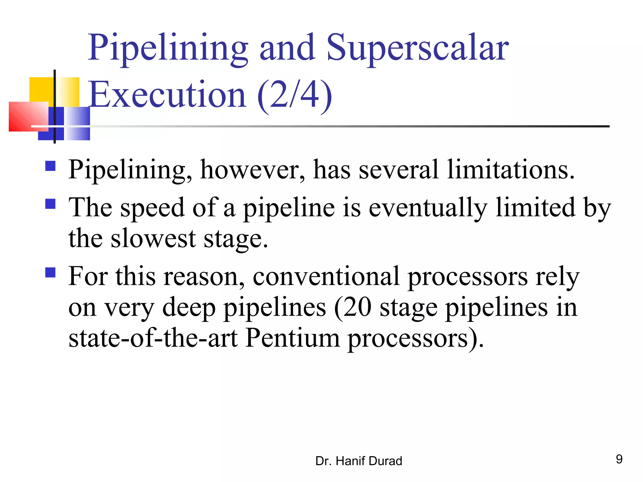
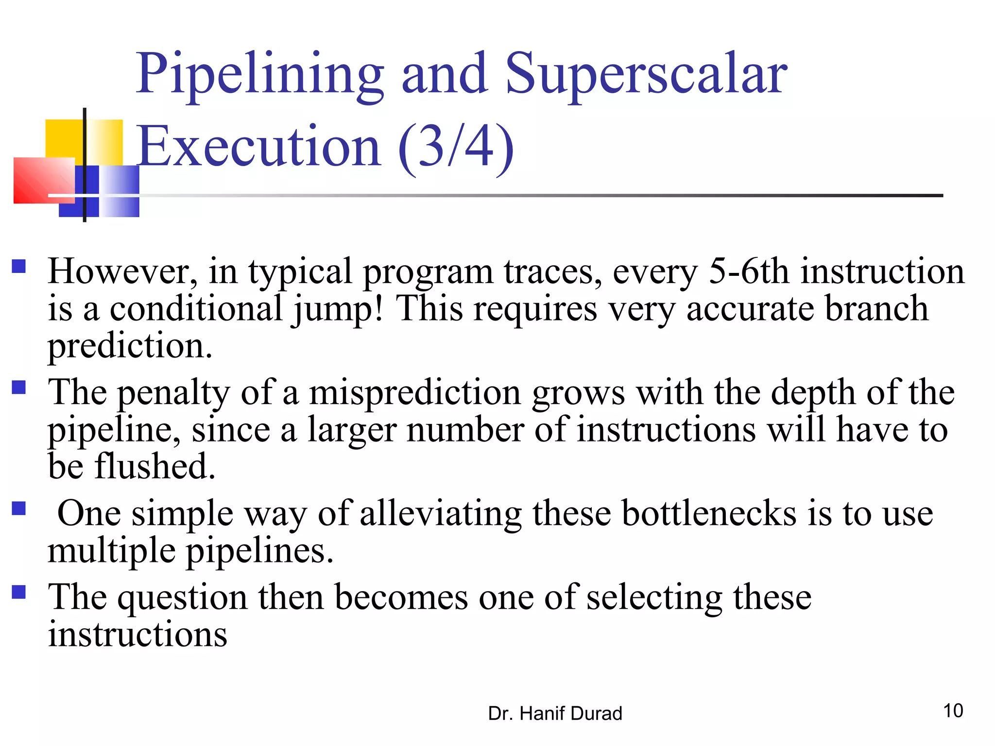
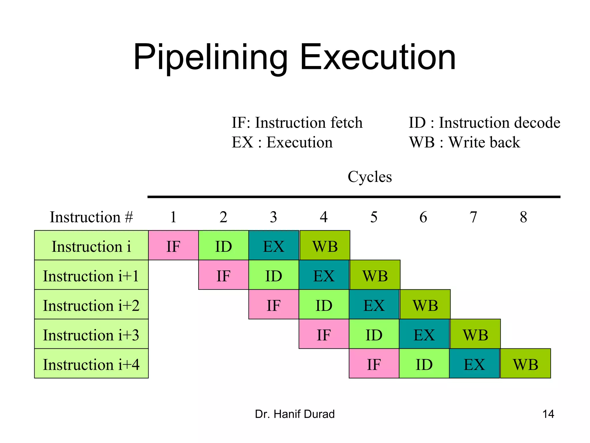
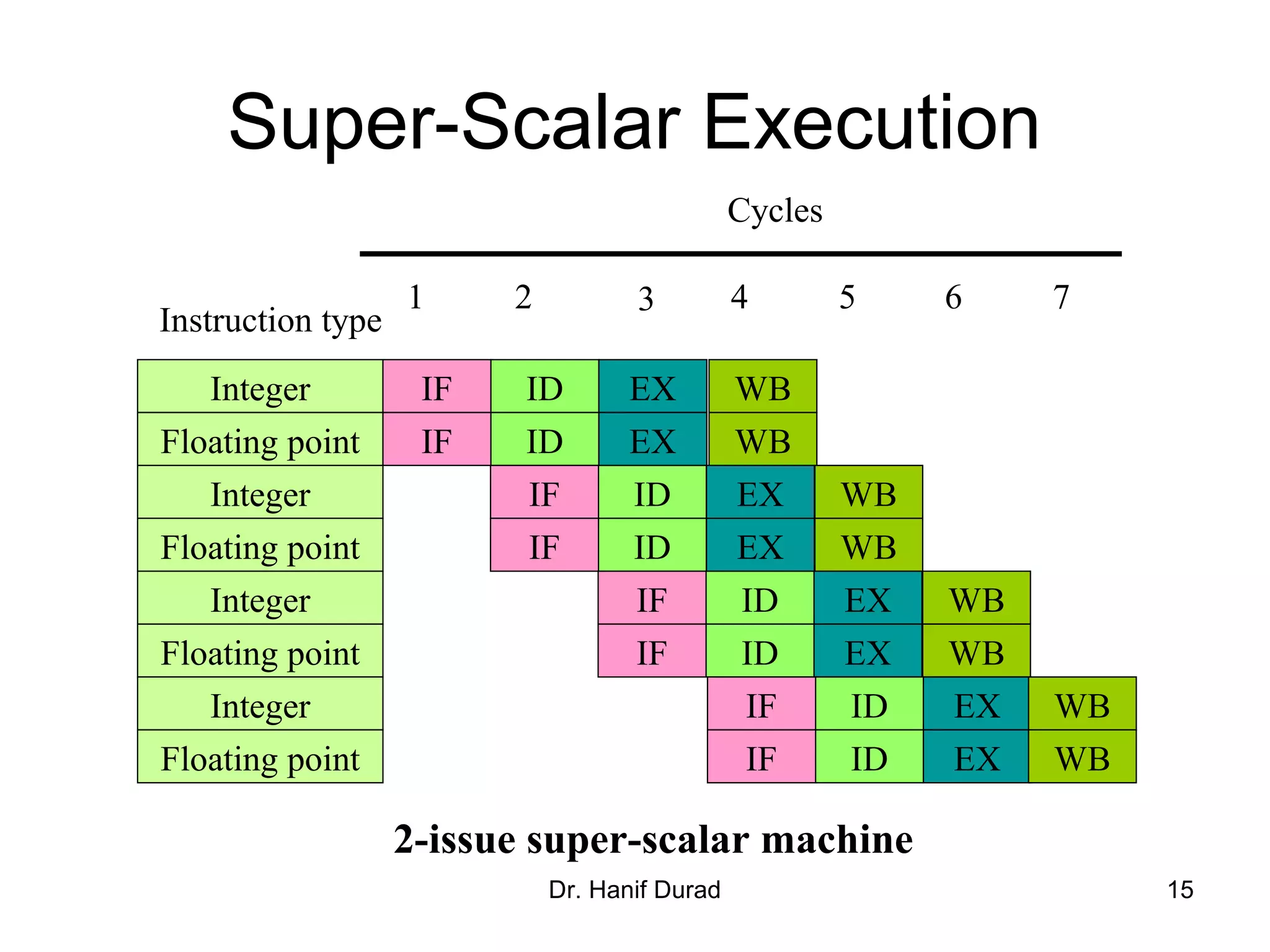
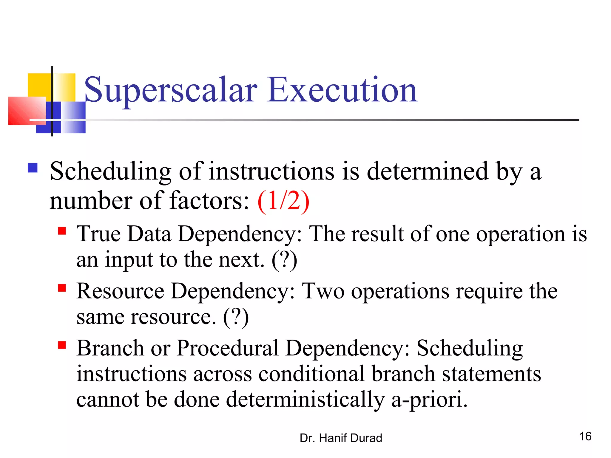
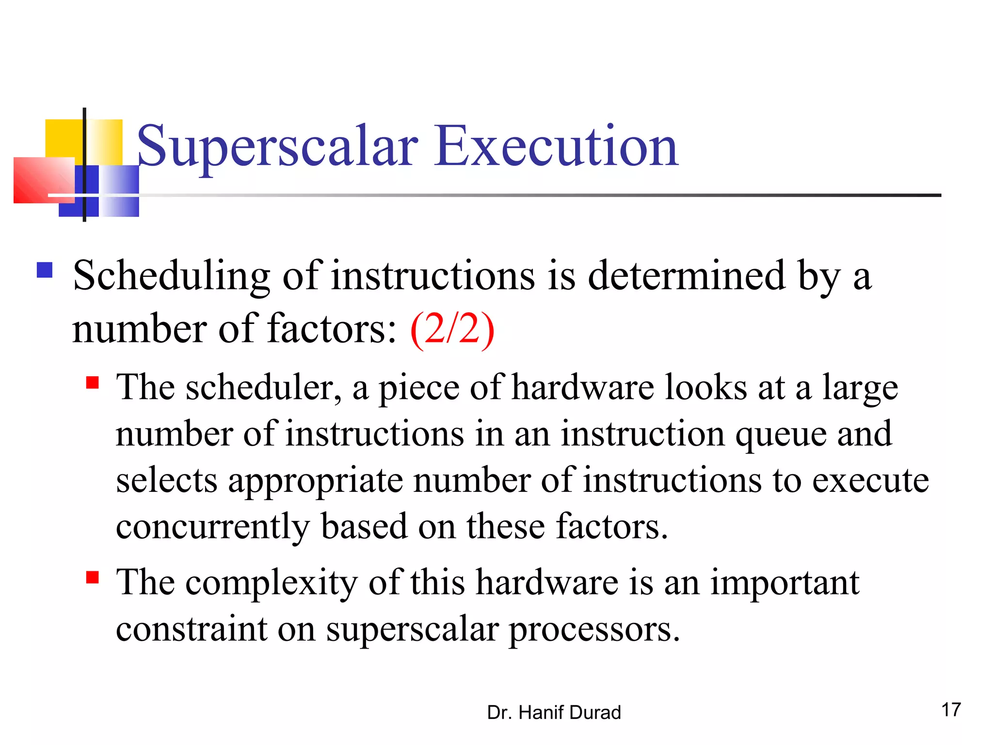
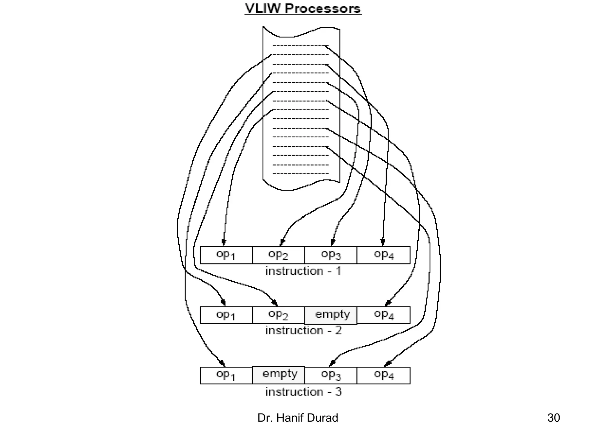
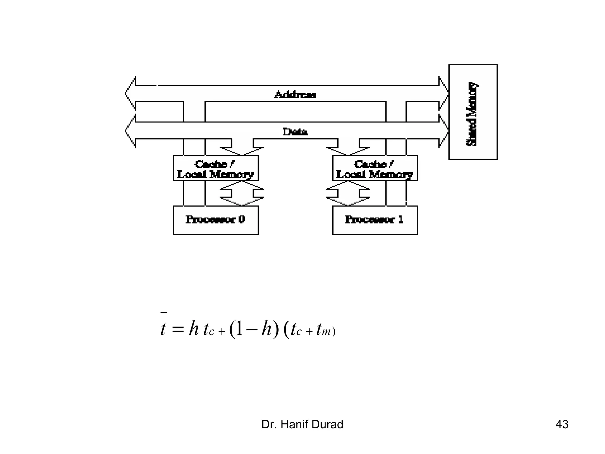
This document provides an outline and overview of parallel computing platforms and trends in microprocessor architectures. It discusses limitations in memory system performance and dichotomy of parallel platforms. Implicit parallelism through techniques like pipelining and superscalar execution aim to improve processor performance by executing multiple instructions concurrently. However, dependencies and other factors limit efficiency. Alternative approaches like VLIW aim to simplify hardware by moving scheduling to compile time. Memory latency and bandwidth are also significant bottlenecks, as data access times are orders of magnitude slower than processor speeds. Overall parallelism seeks to address performance limitations in processors, memory, and communication.