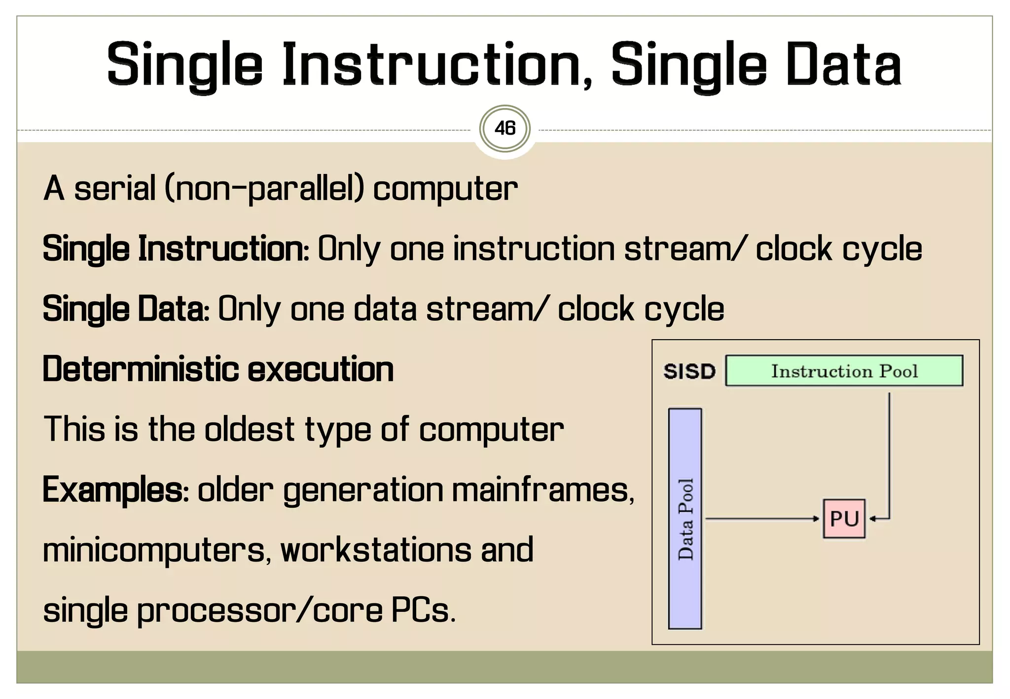
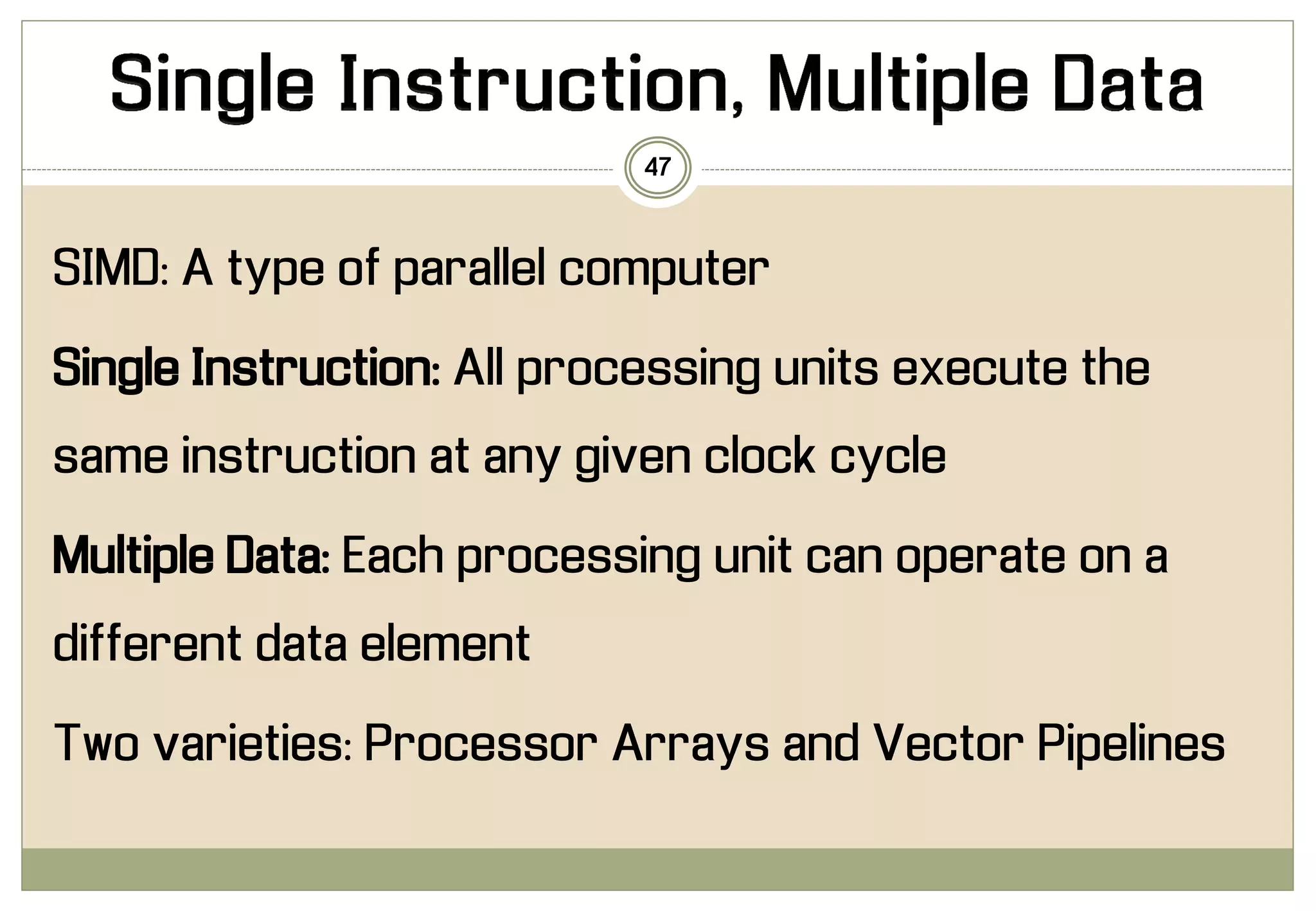
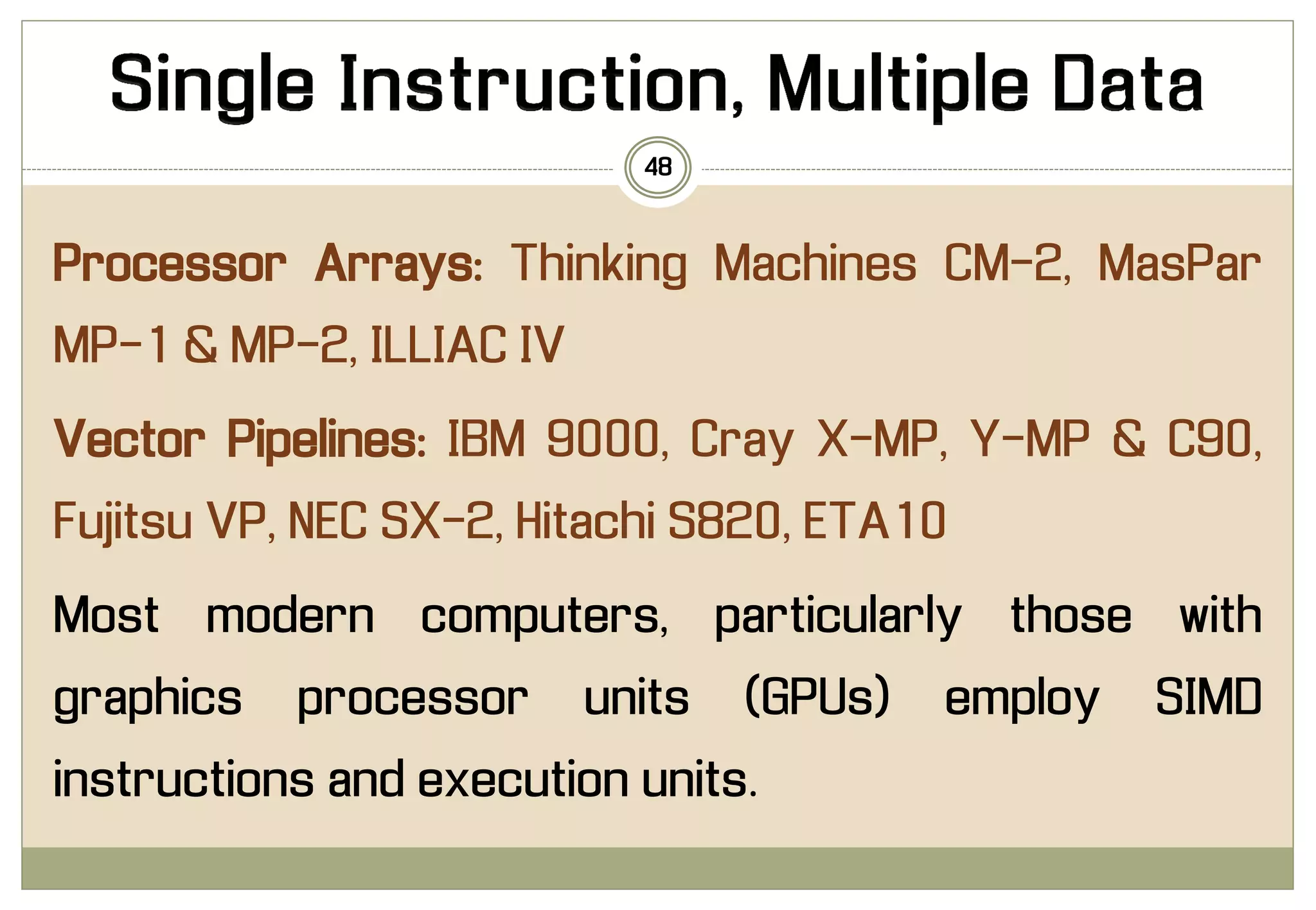
Demand for
High Speed
Computers
2
Demand for High Speed Computers
Technological advancement has its Limits
Solution is Replication of Processing Units
It leads to parallel Computers
3
4
Observations
Theory
Physical
Experiment
Classical science is based on
observation,
theory, and
physical experimentation
Observation of a phenomenon leads
to a hypothesis.
The scientist develops a theory to
explain the phenomenon and designs
an experiment to test that theory.
5
Nature
Physical experiments are not always
feasible because:
• Too Expensive
• Time Consuming
• Unethical
• Impossible to perform
In contrast, modern science is
characterized by observation, theory,
experimentation, and numerical
simulation.
6
Observations
Theory
Numerical
Simulation
Nature
Numerical Simulation creates the experimental environment by using
Mathematical formulas. It is an increasingly important tool for
scientists, who often cannot use physical experiments to test
theories.
The modern scientist compares the behaviour of a numerical
simulation, which implements the theory, to observation of “real world”
phenomena.
Many important scientific problems are so complex that solving them
via numerical simulation requires extraordinarily powerful computers.
7
These complex problems, often called grand challenges
for science (Levin 1989):
• Quantum chemistry, statistical mechanics, and relativistic physics
• Cosmology and astrophysics
• Computational fluid dynamics and turbulence
• Materials design and superconductivity
• Biology, pharmacology, genome sequencing, genetic engineering,
protein folding, enzyme activity, and cell modelling
• Medicine, and modelling of human organs and bones
• Global weather and environmental modelling
8
9
Solomon: constructed by Westinghouse Electric Company in
the early 1960s.
ILLIAC IV: assembled at Burrough Corporation in the early
1970s.
At Carnegie-Mellon University, two parallel computers
C.mmp and Cm* were constructed during 1970s.
In early1980s researchers at Caltech built the parallel
computer Cosmic Cube
In the mid -1980s the parallel commercial computers were
constructed with microprocessors.
It took more than 20 years for parallel computers to move from the lab to market.
10
PP: Parallel Processing
Daniel Slotnick at University of Illinois designed two early parallel computers
11
PP: Parallel Processing
(Credit Hennessy and Patterson)
The performance growth
rate for minicomputers,
mainframes and traditional
supercomputer has been
just under 20% a year
While the performance growth
rate for microprocessors has
averaged 35% a year.
12
PP: Parallel Processing
The performance of Processor can be improved
through
13
PP: Parallel Processing
Fundamental Architectural Advances
Bit parallel
memory
Bit-parallel
arithmetic
Cache
memory
Channels
Interleaved
memory
Instruction
lookahead
Instruction
pipelining
Multiple
functional
units
Pipelined
functional
units
Data
pipelining
14
PP: Parallel Processing
Microprocessors have been able to achieve more
impressive performance gain because-
They are at the
beginning stage
They have not
incorporated all
the architectural
advances
Their clock speed
is much slower
15
PP: Parallel Processing
Microprocessors
Convergence in relative performance between
Supercomputers
Commercial
Parallel
Computers
16
PP: Parallel Processing
Single
processor
Supercomputer
Microprocessor
based parallel
computers
17
PP: Parallel Processing
Some of the organizations that delivered commercial parallel computers based on
microprocessor CPUs in the 10-year period 1984-1993 and their current status.
18
PP: Parallel Processing
Reasonable
Architecture
Operating
Systems
Programming
Languages
Parallel
Algorithms
Harnessing the power
latent in massive
parallel microprocessor
based computers,
however, requires the
development of
19
PP: Parallel Processing
This paper is about the
designing of efficient algorithms
for real parallel computers.
20
PP: Parallel Processing
21
Parallel computing is the use of a parallel computer to
reduce the time needed to solve a single
computational problem.
Parallel computing is now considered a standard way
for computational scientists and engineers to solve
problems in areas as diverse as galactic evolution,
climate modeling, aircraft design, and molecular
dynamics.
22
23
A parallel computer is a multiple processor computer
system supporting parallel programming.
24
Important categories of parallel
computers
Multicomputers Multiprocessors
A multicomputer is a parallel
computer constructed out of
multiple computers and an
interconnection network.
Each computer has its own
memory and it is accessible by
that particular processor .
The processors on different
computers interact by passing
messages to each other.
25
Multiprocessor is a
computer system with two
or more CPUs. It is highly
integrated system in which
all CPUs share access to a
single global memory.
This shared memory supports
communication &
synchronization among
processors.
26
It is information processing that emphasizes the
concurrent manipulation of data elements
belonging to one or more processes solving a
single problem.
A parallel computer capable of parallel processing.
27
• Sequential events or processes which seem to
occur or progress at the same time.
Concurrent Processing
• Events or processes which occur or progress
at the same time
Parallel Processing
28
29
Concurrency: Two or more
threads in progress at the
same time but only one
executed by single CPU.
Parallelism: Two or more
threads executing at the
same time
30
A supercomputer is a general purpose
computer capable of solving individual
problems at extremely high computational
speeds, compared with other computers
built during the same time.
31
The throughput of a devices is the number of
results it produces per unit time.
There are many ways to improve the
throughput of a device.
Speed
By reducing Instruction
Cycle Time
Concurrency
By executing more
instructions per Cycle Time
32
Speedup is the ratio between the time needed
for the most efficient sequential algorithm to
perform a computation and the time needed to
perform the same computation on a machine
incorporating pipelining and/or parallelism.
Speedup = Tsequential/ Tparallel/pipelined
33
A pipelined computation is divided into a number
of steps called segments or stages. The output of
one segment is the input of the next segment.
34
1 2 3 k……
k
dn …… d3 d2, d1
n * k
k + (n-1)
dn …… d3 d2, d1
d1
d1d2
d1d2d3
d1dk-2dk-1dk ……
Speedup = n*k/(k+n-1) lim
𝑛→∞
𝑘 + 𝑛 − 1 → 𝑛, 𝑆𝑝𝑒𝑒𝑑𝑢𝑝 = 𝑘
35
Data Parallelism is the use of multiple functional
units to apply the same operation simultaneously
to element of a data set.
THE SAME SET OF OPERATIONS TO DIFFERENT DATA
36
A k-fold increase in the number of
functional units leads to a k-fold
increase in the throughput of the
system if there is no overhead
associated with the parallelism.
A processor array is a parallel computer with set
of identical, ALUs/Processing Elements (PEs) that
can operate in parallel in a lock step fashion under
the control of one control unit and a number of
memory modules.
37
38
Three methods to assemble widgets.
a) A sequential widget assembly
machine produces one widget
every three units of time.
b) A three segment pipelined widget-
assembly machine produces the
first widget in three units of time
and successive widgets every time
unit thereafter.
c) A three-way data-parallel widget-
assembly machine produces three
widgets every three units of time.
39
No. of
Wi
Seq. Pipelined Parallel
Tsq Tpi Speedup Tpa Speedup
1 3 3 1 3 1
2 6 4 1.5 3 2
3 9 5 1.8 3 3
4 12 6 2 6 2
5 15 7 2.1 6 2.5
6 18 8 2.2 6 3
7 21 9 2.3 9 2.3
8 24 10 2.4 9 2.6
9 27 11 2.4 9 3
10 30 12 2.5 12 2.5
0
0.5
1
1.5
2
2.5
3
3.5
1 2 3 4 5 6 7 8 9 10
Speedup
Widgets Assembled
Pipelined Parallel
Control parallelism is
achieved by applying
different operations to
different data elements
simultaneously.
40
Pipelining is a special case of control parallelism.
Most realistic problems can exploit both data and
control parallelism.
Problem: Weekly maintenance of a Lawn
1. Mowing the Lawn
2. Edging the Lawn
3. Checking the Sprinkle
4. Weeding the flower beds
41
Different workers mowing the
lawn simultaneously
(Data Parallelism)
Other team of workers are
weeding the flower bed in parallel
(Control Parallelism)
42
Turn off
Security
System
Check
Sprinklers
Turn on
Security
System
Mow
Lawn
Edge
Lawn
Weed
Garden
An algorithm is scalable if the level of parallelism increases at
least linearly with the problem size.
An architecture is scalable if it continues to yield the same
performance per processor, albeit used on a larger problem
size, as the number of processors increases.
Data parallel algorithms are more scalable than control
parallel algorithms. Control parallelism is usually a constant,
independent of the problem size, while the level of data
parallelism is an increasing function of the problem size.
43
There are different ways to classify parallel computers. One of the
more widely used classifications, in use since 1966, is called
Flynn's Taxonomy.
Flynn's taxonomy distinguishes multi-processor computer
architectures according to how they can be classified along the
two independent dimensions of Instruction Stream and Data
Stream. Each of these dimensions can have only one of two
possible states: Single or Multiple.
44
45
A serial (non-parallel) computer
Single Instruction: Only one instruction stream/ clock cycle
Single Data: Only one data stream/ clock cycle
Deterministic execution
This is the oldest type of computer
Examples: older generation mainframes,
minicomputers, workstations and
single processor/core PCs.
46
SIMD: A type of parallel computer
Single Instruction: All processing units execute the
same instruction at any given clock cycle
Multiple Data: Each processing unit can operate on a
different data element
Two varieties: Processor Arrays and Vector Pipelines
47
Processor Arrays: Thinking Machines CM-2, MasPar
MP-1 & MP-2, ILLIAC IV
Vector Pipelines: IBM 9000, Cray X-MP, Y-MP & C90,
Fujitsu VP, NEC SX-2, Hitachi S820, ETA10
Most modern computers, particularly those with
graphics processor units (GPUs) employ SIMD
instructions and execution units.
48
49
50
(MISD): A type of parallel computer
Multiple Instruction: Each processing unit operates on the
data independently via separate instruction streams.
Single Data: A single data stream is fed into multiple
processing units.
Few (if any) actual examples of this class of parallel
computer have ever existed.
51
(MIMD): A type of parallel computer
Multiple Instruction: Every processor may be
executing a different instruction stream
Multiple Data: Every processor may be working with a
different data stream
The most common type of parallel computer - most
modern supercomputers fall into this category.
52
Examples:
most current
supercomputers, networked
parallel computer clusters
and "grids", multi-processor
SMP computers, multi-core
PCs.
53 Topic Covered in the Presentation
Chapter 1: Introduction
1.1 Computational Demands of Modern Science
1.2 Advent of Practical Parallel Processing
1.3 Parallel Processing Terminology

Chapter 1 - introduction - parallel computing

  • 2.
  • 3.
    Demand for HighSpeed Computers Technological advancement has its Limits Solution is Replication of Processing Units It leads to parallel Computers 3
  • 4.
  • 5.
    Observations Theory Physical Experiment Classical science isbased on observation, theory, and physical experimentation Observation of a phenomenon leads to a hypothesis. The scientist develops a theory to explain the phenomenon and designs an experiment to test that theory. 5 Nature
  • 6.
    Physical experiments arenot always feasible because: • Too Expensive • Time Consuming • Unethical • Impossible to perform In contrast, modern science is characterized by observation, theory, experimentation, and numerical simulation. 6 Observations Theory Numerical Simulation Nature
  • 7.
    Numerical Simulation createsthe experimental environment by using Mathematical formulas. It is an increasingly important tool for scientists, who often cannot use physical experiments to test theories. The modern scientist compares the behaviour of a numerical simulation, which implements the theory, to observation of “real world” phenomena. Many important scientific problems are so complex that solving them via numerical simulation requires extraordinarily powerful computers. 7
  • 8.
    These complex problems,often called grand challenges for science (Levin 1989): • Quantum chemistry, statistical mechanics, and relativistic physics • Cosmology and astrophysics • Computational fluid dynamics and turbulence • Materials design and superconductivity • Biology, pharmacology, genome sequencing, genetic engineering, protein folding, enzyme activity, and cell modelling • Medicine, and modelling of human organs and bones • Global weather and environmental modelling 8
  • 9.
  • 10.
    Solomon: constructed byWestinghouse Electric Company in the early 1960s. ILLIAC IV: assembled at Burrough Corporation in the early 1970s. At Carnegie-Mellon University, two parallel computers C.mmp and Cm* were constructed during 1970s. In early1980s researchers at Caltech built the parallel computer Cosmic Cube In the mid -1980s the parallel commercial computers were constructed with microprocessors. It took more than 20 years for parallel computers to move from the lab to market. 10 PP: Parallel Processing Daniel Slotnick at University of Illinois designed two early parallel computers
  • 11.
    11 PP: Parallel Processing (CreditHennessy and Patterson)
  • 12.
    The performance growth ratefor minicomputers, mainframes and traditional supercomputer has been just under 20% a year While the performance growth rate for microprocessors has averaged 35% a year. 12 PP: Parallel Processing
  • 13.
    The performance ofProcessor can be improved through 13 PP: Parallel Processing
  • 14.
    Fundamental Architectural Advances Bitparallel memory Bit-parallel arithmetic Cache memory Channels Interleaved memory Instruction lookahead Instruction pipelining Multiple functional units Pipelined functional units Data pipelining 14 PP: Parallel Processing
  • 15.
    Microprocessors have beenable to achieve more impressive performance gain because- They are at the beginning stage They have not incorporated all the architectural advances Their clock speed is much slower 15 PP: Parallel Processing
  • 16.
    Microprocessors Convergence in relativeperformance between Supercomputers Commercial Parallel Computers 16 PP: Parallel Processing
  • 17.
  • 18.
    Some of theorganizations that delivered commercial parallel computers based on microprocessor CPUs in the 10-year period 1984-1993 and their current status. 18 PP: Parallel Processing
  • 19.
    Reasonable Architecture Operating Systems Programming Languages Parallel Algorithms Harnessing the power latentin massive parallel microprocessor based computers, however, requires the development of 19 PP: Parallel Processing
  • 20.
    This paper isabout the designing of efficient algorithms for real parallel computers. 20 PP: Parallel Processing
  • 21.
  • 22.
    Parallel computing isthe use of a parallel computer to reduce the time needed to solve a single computational problem. Parallel computing is now considered a standard way for computational scientists and engineers to solve problems in areas as diverse as galactic evolution, climate modeling, aircraft design, and molecular dynamics. 22
  • 23.
  • 24.
    A parallel computeris a multiple processor computer system supporting parallel programming. 24 Important categories of parallel computers Multicomputers Multiprocessors
  • 25.
    A multicomputer isa parallel computer constructed out of multiple computers and an interconnection network. Each computer has its own memory and it is accessible by that particular processor . The processors on different computers interact by passing messages to each other. 25
  • 26.
    Multiprocessor is a computersystem with two or more CPUs. It is highly integrated system in which all CPUs share access to a single global memory. This shared memory supports communication & synchronization among processors. 26
  • 27.
    It is informationprocessing that emphasizes the concurrent manipulation of data elements belonging to one or more processes solving a single problem. A parallel computer capable of parallel processing. 27
  • 28.
    • Sequential eventsor processes which seem to occur or progress at the same time. Concurrent Processing • Events or processes which occur or progress at the same time Parallel Processing 28
  • 29.
    29 Concurrency: Two ormore threads in progress at the same time but only one executed by single CPU. Parallelism: Two or more threads executing at the same time
  • 30.
    30 A supercomputer isa general purpose computer capable of solving individual problems at extremely high computational speeds, compared with other computers built during the same time.
  • 31.
    31 The throughput ofa devices is the number of results it produces per unit time. There are many ways to improve the throughput of a device. Speed By reducing Instruction Cycle Time Concurrency By executing more instructions per Cycle Time
  • 32.
    32 Speedup is theratio between the time needed for the most efficient sequential algorithm to perform a computation and the time needed to perform the same computation on a machine incorporating pipelining and/or parallelism. Speedup = Tsequential/ Tparallel/pipelined
  • 33.
    33 A pipelined computationis divided into a number of steps called segments or stages. The output of one segment is the input of the next segment.
  • 34.
    34 1 2 3k…… k dn …… d3 d2, d1 n * k k + (n-1) dn …… d3 d2, d1 d1 d1d2 d1d2d3 d1dk-2dk-1dk …… Speedup = n*k/(k+n-1) lim 𝑛→∞ 𝑘 + 𝑛 − 1 → 𝑛, 𝑆𝑝𝑒𝑒𝑑𝑢𝑝 = 𝑘
  • 35.
    35 Data Parallelism isthe use of multiple functional units to apply the same operation simultaneously to element of a data set. THE SAME SET OF OPERATIONS TO DIFFERENT DATA
  • 36.
    36 A k-fold increasein the number of functional units leads to a k-fold increase in the throughput of the system if there is no overhead associated with the parallelism.
  • 37.
    A processor arrayis a parallel computer with set of identical, ALUs/Processing Elements (PEs) that can operate in parallel in a lock step fashion under the control of one control unit and a number of memory modules. 37
  • 38.
    38 Three methods toassemble widgets. a) A sequential widget assembly machine produces one widget every three units of time. b) A three segment pipelined widget- assembly machine produces the first widget in three units of time and successive widgets every time unit thereafter. c) A three-way data-parallel widget- assembly machine produces three widgets every three units of time.
  • 39.
    39 No. of Wi Seq. PipelinedParallel Tsq Tpi Speedup Tpa Speedup 1 3 3 1 3 1 2 6 4 1.5 3 2 3 9 5 1.8 3 3 4 12 6 2 6 2 5 15 7 2.1 6 2.5 6 18 8 2.2 6 3 7 21 9 2.3 9 2.3 8 24 10 2.4 9 2.6 9 27 11 2.4 9 3 10 30 12 2.5 12 2.5 0 0.5 1 1.5 2 2.5 3 3.5 1 2 3 4 5 6 7 8 9 10 Speedup Widgets Assembled Pipelined Parallel
  • 40.
    Control parallelism is achievedby applying different operations to different data elements simultaneously. 40 Pipelining is a special case of control parallelism.
  • 41.
    Most realistic problemscan exploit both data and control parallelism. Problem: Weekly maintenance of a Lawn 1. Mowing the Lawn 2. Edging the Lawn 3. Checking the Sprinkle 4. Weeding the flower beds 41
  • 42.
    Different workers mowingthe lawn simultaneously (Data Parallelism) Other team of workers are weeding the flower bed in parallel (Control Parallelism) 42 Turn off Security System Check Sprinklers Turn on Security System Mow Lawn Edge Lawn Weed Garden
  • 43.
    An algorithm isscalable if the level of parallelism increases at least linearly with the problem size. An architecture is scalable if it continues to yield the same performance per processor, albeit used on a larger problem size, as the number of processors increases. Data parallel algorithms are more scalable than control parallel algorithms. Control parallelism is usually a constant, independent of the problem size, while the level of data parallelism is an increasing function of the problem size. 43
  • 44.
    There are differentways to classify parallel computers. One of the more widely used classifications, in use since 1966, is called Flynn's Taxonomy. Flynn's taxonomy distinguishes multi-processor computer architectures according to how they can be classified along the two independent dimensions of Instruction Stream and Data Stream. Each of these dimensions can have only one of two possible states: Single or Multiple. 44
  • 45.
  • 46.
    A serial (non-parallel)computer Single Instruction: Only one instruction stream/ clock cycle Single Data: Only one data stream/ clock cycle Deterministic execution This is the oldest type of computer Examples: older generation mainframes, minicomputers, workstations and single processor/core PCs. 46
  • 47.
    SIMD: A typeof parallel computer Single Instruction: All processing units execute the same instruction at any given clock cycle Multiple Data: Each processing unit can operate on a different data element Two varieties: Processor Arrays and Vector Pipelines 47
  • 48.
    Processor Arrays: ThinkingMachines CM-2, MasPar MP-1 & MP-2, ILLIAC IV Vector Pipelines: IBM 9000, Cray X-MP, Y-MP & C90, Fujitsu VP, NEC SX-2, Hitachi S820, ETA10 Most modern computers, particularly those with graphics processor units (GPUs) employ SIMD instructions and execution units. 48
  • 49.
  • 50.
    50 (MISD): A typeof parallel computer Multiple Instruction: Each processing unit operates on the data independently via separate instruction streams. Single Data: A single data stream is fed into multiple processing units. Few (if any) actual examples of this class of parallel computer have ever existed.
  • 51.
    51 (MIMD): A typeof parallel computer Multiple Instruction: Every processor may be executing a different instruction stream Multiple Data: Every processor may be working with a different data stream The most common type of parallel computer - most modern supercomputers fall into this category.
  • 52.
    52 Examples: most current supercomputers, networked parallelcomputer clusters and "grids", multi-processor SMP computers, multi-core PCs.
  • 53.
    53 Topic Coveredin the Presentation Chapter 1: Introduction 1.1 Computational Demands of Modern Science 1.2 Advent of Practical Parallel Processing 1.3 Parallel Processing Terminology